9.1 Distribution of the Difference between Two Sample Means for Two Independent Samples
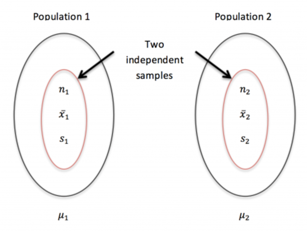
Suppose two populations have means [latex]\mu_1[/latex], [latex]\mu_2[/latex] and standard deviations [latex]\sigma_1[/latex], [latex]\sigma_2[/latex]. Further, suppose that we obtain from each population simple random samples, from which we obtain sample means [latex]\bar{x}_1[/latex] and [latex]\bar{x}_2[/latex]. Our objective is to make inferences about [latex]\mu_1[/latex] – [latex]\mu_2[/latex] using the unbiased estimate [latex]\bar{x}_1[/latex] - [latex]\bar{x}_2[/latex] and as such, we need to know the distribution of [latex]\bar{X}_1 - \bar{X}_2[/latex].
Recall the conclusions about the sampling distribution of the sample mean [latex]\bar{X}[/latex] based on samples of size n taken from a population with mean [latex]\mu[/latex] and standard deviation [latex]\sigma[/latex]:
- The mean of [latex]\bar{X}[/latex] equals the population mean [latex]\mu[/latex], i.e., [latex]\mu_{\scriptsize \bar{X}} = \mu[/latex].
- The standard deviation of [latex]\bar{X}[/latex] equals the population standard deviation divided by the square root of the sample size n, i.e., [latex]\sigma_{\scriptsize\bar{X}} = \frac{\sigma}{\sqrt{n}}[/latex].
These two conclusions are always true regardless of the population distribution and the sample size n. - The shape of the distribution of [latex]\bar{X}[/latex]:
- If the population is normally distributed, so is [latex]\bar{X}[/latex] regardless of the sample size n.
- If the population is not normally distributed, but the sample size n is relatively large, say [latex]n \geq 30[/latex], then the sample mean [latex]\bar{X}[/latex] is approximately normally distributed.
A similar idea applies to the distribution of [latex]\bar{X_1} - \bar{X_2}[/latex].
Key Facts: Sampling Distribution of [latex]\color{white}\bar{X_1}-\bar{X_2}[/latex]
- The mean of [latex]\bar{X_1} - \bar{X_2}[/latex] equals the difference of the population means: [latex]\mu_{\scriptsize \bar{X_1} - \bar{X_2}} = \mu_1 - \mu_2[/latex].
- The standard deviation of [latex]\bar{X_1} - \bar{X_2}[/latex] is: [latex]\sigma_{\scriptsize \bar{X_1} - \bar{X_2}} = \sqrt{\frac{\sigma_1^2}{n_1} + \frac{\sigma_2^2}{n_2}}[/latex].
These two conclusions are always true regardless of the population distributions and the sample sizes [latex]n_1[/latex] and [latex]n_2[/latex]. - The shape of the distribution of [latex]\bar{X_1} - \bar{X_2}[/latex]:
- If the populations are normally distributed, [latex]\bar{X_1} - \bar{X_2}[/latex] is exactly normally distributed regardless of the sample sizes [latex]n_1[/latex] and [latex]n_2[/latex].
- If the populations are not normally distributed, but sample sizes [latex]n_1[/latex] and [latex]n_2[/latex] are relatively large, say [latex]n_1 \geq 30[/latex] and [latex]n_2 \geq 30[/latex], then by the central limit theorem both [latex]\bar{X_1}[/latex] and [latex]\bar{X_2}[/latex] are approximately normally distributed. The difference of two normal distributions is still normal; therefore, for [latex]n_1 \geq 30[/latex] and [latex]n_2 \geq 30[/latex], [latex]\bar{X_1} - \bar{X_2}[/latex] is approximately normally distributed.
To summarize, for normal populations OR large sample sizes
[latex]\bar{X_1} - \bar{X_2} \sim N \left( \mu_1 - \mu_2, \sqrt{ \frac{\sigma_1^2}{n_1} + \frac{\sigma_2^2}{n_2}} \right).[/latex]
We can also standardize [latex]\bar{X_1} - \bar{X_2}[/latex] to convert it into a standard normal random variable:
[latex]Z = \frac{(\bar{X_1} - \bar{X_2}) - (\mu_1 - \mu_2)}{\sqrt{ \frac{\sigma_1^2}{n_1} + \frac{\sigma_2^2}{n_2}}} \sim N(0, 1).[/latex]
If the population standard deviations [latex]\sigma_1[/latex] and [latex]\sigma_2[/latex] are unknown and estimated by sample standard deviations [latex]s_1[/latex] and [latex]s_2[/latex], the studentized version of [latex]\bar{X_1} - \bar{X_2}[/latex] is
[latex]t = \frac{(\bar{X_1} - \bar{X_2}) - (\mu_1 - \mu_2)}{\sqrt{ \frac{s_1^2}{n_1} + \frac{s_2^2}{n_2}}} \sim t \text{ distribution}[/latex]
with degrees of freedom
[latex]df = \frac{ \left( \frac{s_1^2}{n_1} + \frac{s_2^2}{n_2} \right)^2}{\frac{1}{n_1 - 1} \left( \frac{s_1^2}{n_1} \right)^2 + \frac{1}{n_2 - 1} \left( \frac{s_2^2}{n_2} \right)^2 } \text{ rounded down to the nearest integer}.[/latex]

The degrees of freedom calculation given in the above equation is very complicated, so for exams, you can use the conservative lower bound, which is defined as the smaller value of [latex]n_1 - 1[/latex] and [latex]n_2 - 1[/latex]. That is, you may use [latex]df = \min\{n_1 -1, n_2 - 1 \}[/latex].
For example, if [latex]n_1 = 40, n_2 = 50[/latex], then [latex]df = \min\{n_1 -1, n_2 - 1 \} = \min\{40-1, 50-1 \} = \min\{39, 49 \} = 39.[/latex]
