5.3 Standard Normal Density Curve
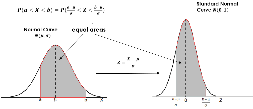
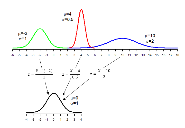
The standardized variable (z-score) has a mean of 0 and a standard deviation of 1. We can also standardize the normal variable [latex]X \sim N(\mu, \sigma)[/latex] by [latex]Z=\frac{X - \mu}{\sigma}[/latex] and [latex]Z[/latex] follows a standard normal distribution with mean 0 and standard deviation 1, i.e., [latex]Z \sim N(0,1)[/latex].
The standard normal density curve has the following properties:
Key Facts: Properties of a Standard Normal Density Curve
- Total area under the curve is 1.
- The curve extends from [latex]- \infty[/latex] to [latex]+ \infty[/latex].
- Symmetric at 0, which means the area to the right of a positive number [latex]a[/latex] is equal to the area to the left of [latex]-a[/latex]. For example, [latex]P(Z \ge 2) = P(Z \le -2).[/latex]
- Empirical rule:
- 68.26% of the observations are within the interval [-1, 1]. The area under the curve between -1 and 1 is 0.6826.
- 95.44% of the observations are within the interval [-2, 2]. The area under the curve between -2 and 2 is 0.9544.
- 99.74% of the observations are within the interval [-3, 3]. The area under the curve between -3 and 3 is 0.9974.
Standardization converts all normal distributions to a single one—the standard normal distribution. Therefore, we can calculate the probabilities of events relative to any normal distribution using only the standard normal density curve.
Example: Density Curve and Probability
Suppose the grades in a Statistics class are approximately normally distributed with mean [latex]\mu=70[/latex] and standard deviation [latex]\sigma=10[/latex].
- The percentage (proportion, to be more precise) of students with a grade below 60 equals the area under the standard normal curve to the left of -1. The [latex]z[/latex]-score is calculated by [latex]z = \frac{x- \mu}{\sigma} = \frac{60 - 70}{10} = -1[/latex].
- The percentage (proportion) of students with a grade above 90 equals the area under the standard normal curve to the right of 2. The [latex]z[/latex]-score is calculated by [latex]z = \frac{x- \mu}{\sigma} = \frac{90 - 70}{10} = 2[/latex].
- The percentage (proportion) of students with a grade between 60 and 90 equals the area under the standard normal curve between -1 and 2. Figure 5.4 gives a graphical presentation of this question with [latex]\mu=70, \sigma=10, a=60[/latex] and [latex]b=90[/latex].
