13.9 Confidence Intervals and Prediction Intervals
Suppose the model assumptions are satisfied and the regression model fits the data. In that case, we can use the fitted least-squares regression model to estimate the conditional mean [latex]\mu_p[/latex] and a single value of the response variable [latex]y_p[/latex], corresponding to an observed value of the predictor variable [latex]x_p[/latex]. For example, we can predict the mean price of all used cars that are seven years old and we can use this predicted value to construct a confidence interval for the mean price of all used cars of this age. We can also predict the price of a single used car that is seven years old and construct a so-called prediction interval for the price of a single used car of this age.
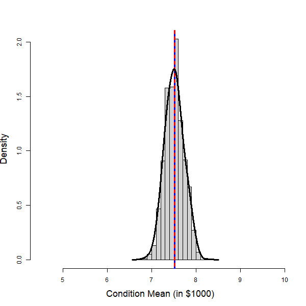
Given a fixed value of the predictor variable, [latex]x = x_p[/latex], a point estimate for the conditional mean [latex]\mu_p = \beta_0 + \beta_1 x_p[/latex] is given by [latex]\hat{\mu}_p = b_0 + b_1 x_p[/latex]. It can be shown that the conditional mean [latex]\hat{\mu}_p[/latex] follows a normal distribution with mean [latex]\mu_p[/latex] and with a standard deviation [latex]SD(\hat{\mu}_p) = \sigma \sqrt{\frac{(x_p - \bar{x})^2}{S_{xx}} + \frac{1}{n}}[/latex], i.e., [latex]\hat{\mu}_p \sim N(\mu_p, \sigma \sqrt{\frac{(x_p - \bar{x})^2}{S_{xx}} + \frac{1}{n}})[/latex]. In the following figure, the histogram in the left panel shows the distribution of the mean price of used cars that are seven years old, based on 1,000 simple random samples of size [latex]n = 15[/latex]. The distribution is roughly normal. The common standard deviation of the error term is estimated by the residual sample standard deviation [latex]s_e[/latex]. Therefore,
[latex]\frac{\hat{\mu}_p - (\beta_0 + \beta_1 x_p)}{\sigma \sqrt{ \frac{(x_p - \bar{x})^2}{S_{xx}} + \frac{1}{n} + 1}} \sim N(0, 1)[/latex] and [latex]\frac{\hat{\mu}_p - (\beta_0 + \beta_1 x_p)}{s_e \sqrt{ \frac{(x_p - \bar{x})^2}{S_{xx}} + \frac{1}{n} + 1}} \sim t[/latex] with [latex]df = n-2[/latex].
A [latex](1 - \alpha) \times 100 \%[/latex] confidence interval for the conditional mean [latex]\mu_p[/latex] is
[latex]\hat{\mu}_p \pm t_{\alpha / 2} \times SE(\hat{\mu}_p) = (b_0 + b_1 x_p) \pm t_{\alpha / 2} \times s_e \sqrt{\frac{(x_p - \bar{x})^2}{S_{xx}} + \frac{1}{n}}[/latex].
A single value of the response variable, given the value of the predictor variable [latex]x = x_p[/latex] can be modeled by [latex]y_p = \beta_0 = \beta_1 x_p + \epsilon[/latex], [latex]\epsilon \sim N(0, \sigma)[/latex]. A point estimate for [latex]y_p[/latex] is given by [latex]\hat{y}_p = b_0 + b_1 x_p,[/latex] which is the same as the point estimate for the conditional mean [latex]\hat{\mu}_p[/latex]. It can be shown that the predicted value for a single response [latex]\hat{y}_p[/latex] follows a normal distribution with mean [latex](\beta_0 + \beta_1 x_p)[/latex] and with a standard deviation [latex]SD(\hat{y}_p) = \sigma \sqrt{\frac{(x_p - \bar{x})^2}{S_{xx}}+\frac{1}{n} + 1}[/latex], i.e.,
[latex]\hat{y}_p \sim N\left(\beta_0 + \beta_1 x_p , \sigma \sqrt{\frac{(x_p - \bar{x})^2}{S_{xx}}+\frac{1}{n} + 1}\right).[/latex]
In the following figure, the histogram in the right panel shows the distribution of the price of a randomly selected used car that is seven years old. The distribution is roughly normal. Therefore,
[latex]\frac{\hat{\mu}_p - (\beta_0 + \beta_1 x_p)}{\sigma \sqrt{ \frac{(x_p - \bar{x})^2}{S_{xx}} + \frac{1}{n} + 1}} \sim N(0, 1)[/latex] and [latex]\frac{\hat{\mu}_p - (\beta_0 + \beta_1 x_p)}{s_e \sqrt{ \frac{(x_p - \bar{x})^2}{S_{xx}} + \frac{1}{n} + 1}} \sim t[/latex] with [latex]df = n-2[/latex].
A [latex](1 - \alpha ) \times 100\%[/latex] confidence interval for a single response [latex]\hat{y}_p[/latex] is
[latex]\hat{y}_p \pm t_{\alpha / 2} \times SE(\hat{y}_p) = (b_0 + b_1 x_p) \pm t_{\alpha / 2} \times s_e \sqrt{ \frac{(x_p - \bar{x})^2}{S_{xx}} + \frac{1}{n} + 1}[/latex].
We call this interval the prediction interval to distinguish between confidence intervals for the conditional mean versus confidence intervals for a single response.
| Distribution for the Conditional Mean [latex]\hat{\mu}_p = b_0 + b_1 x_p[/latex]
|
Distribution of a single value response [latex]\hat{y}_p = b_0 + b_1 x_p[/latex]
|
| Figure 13.13: Distribution of the Conditional Mean (Left) and a Single Response (Right). [Image Description (See Appendix D Figure 13.13)] Click on the image to enlarge it.
|
|

Example: Confidence Interval and Prediction Interval
Recall the used car example. We have summaries:
[latex]n = 15, \sum x_i = 92, \sum x_i^2 = 724, \sum y_i = 125, \sum y_i^2 = 1193, \sum x_i y_i = 616[/latex],
[latex]S_{xy} = \sum x_i y_i - \frac{\left( \sum x_i \right) \left( \sum y_i \right) }{n} = 616 - \frac{92 \times 125}{15} = -150.667[/latex]
[latex]S_{xx} = \sum x_i^2 - \frac{ \left( \sum x_i \right)^2 }{n} = 724 - \frac{92^2}{15} = 159.733[/latex]
[latex]S_{yy} = \sum y_i^2 - \frac{ \left( \sum y_i \right)^2 }{n} = 1193 - \frac{125^2}{15} = 151.333[/latex]
[latex]b_1 = \frac{S_{xy}}{S_{xx}} = \frac{-150.667}{159.733} = -0.9432[/latex]
[latex]b_0 = \bar{y} - b_1 \bar{x} = \frac{\sum y_i}{n} - b_1 \frac{\sum x_i}{n} = \frac{125}{15} - (- 0.9432) \times \frac{92}{15} = 14.118[/latex].
The least-squares regression line is [latex]\hat{y} = b_0 + b_1 x = 14.118 - 0.9432 \times \text{age}[/latex].
[latex]SSE = S_{yy} - b_1 S_{xy} = 151.333 - (-0.9432) \times (-150.667) = 9.224[/latex]
[latex]s_e = \sqrt{\frac{SSE}{n-2}} = \sqrt{\frac{9.224}{13}} = 0.842.[/latex]
- Construct a 95% confidence interval for the mean price for all used cars that are 7 years old.[latex]df = n-2 = 13, \alpha = 0.05, t_{\alpha / 2} = t_{0.025} , x_p = 7, \bar{x} = \frac{\sum x_i}{n} = \frac{92}{15} = 6.133[/latex]. Hence, the 95% confidence interval for the mean price is
[latex]\begin{align*}&(b_0 + b_1 x_p) \pm t_{\alpha / 2} \times s_e \sqrt{\frac{(x_p - \bar{x})^2}{S_{xx}} + \frac{1}{n}} \\ = & (14.118 - 0.9432 \times 7) \pm 2.160 \times 0.842 \times \sqrt{\frac{(7 - 6.113)^2}{159.733} + \frac{1}{15}} \\ = & (7.030, 8.002).\end{align*}[/latex]
Interpretation: We are 95% confident that the mean price of all 7-year-old cars is somewhere between $7,030 and $8,002.
- Obtain a 95% prediction interval for the sale price of a randomly selected used car that is 7 years old.
The 95% prediction interval for the price of a single car is[latex]\begin{align*}&(b_0 + b_1 x_p) \pm t_{\alpha / 2} \times s_e \sqrt{\frac{(x_p - \bar{x})^2}{S_{xx}} + \frac{1}{n} + 1} \\ =& (14.118 - 0.9432 \times 7) \pm 2.160 \times 0.842 \times \sqrt{\frac{(7 - 6.113)^2}{159.733} + \frac{1}{15} + 1} \\ =& (5.633, 9.398).\end{align*}[/latex]
Interpretation: We are 95% confident that the price of a randomly selected 7-year-old car is somewhere between $5,633 and $9,398.
- Which interval is wider? Explain why.
The prediction interval for a single predicted value is wider than the confidence interval for the conditional mean. This is because the error in predicting the price of a particular 7-year-old used car is due to the error in estimating the regression line plus the variation in prices of all 7-year-old cars. In contrast, the error in predicting the mean price of all 7-year-old cars is only due to the error in estimating the regression line.

Exercise: Application of Simple Linear Regression
An instructor asked a random sample of eight students to record their study times in an introductory calculus course. The total hours studied ([latex]x[/latex]) over two weeks and the test scores ([latex]y[/latex]) at the end of the two weeks are given in the following table.
Table 13.3: Test Score and Study Hour for Eight Students
| Hours ([latex]x[/latex]) |
10
|
15
|
12
|
20
|
8
|
16
|
14
|
22
|
|---|---|---|---|---|---|---|---|---|
| Score ([latex]y[/latex]) |
92
|
81
|
84
|
74
|
85
|
80
|
84
|
80
|
The summaries of the data are given by
[latex]n = 8, \sum x_i = 117, \sum x_i^2 = 1869, \\ \sum y_i = 660 , \sum y_i^2 = 54638, \sum x_i y_i = 9519.[/latex]
- Given the summaries of the data, find the least-squares regression equation.
- Interpret the slope of the regression equation obtained in part a) in the context of the study.
- Calculate and interpret [latex]r[/latex], the correlation coefficient between [latex]y[/latex] and [latex]x[/latex].
- Calculate and interpret the coefficient of determination [latex]r^2[/latex].
- Test at the 5% significant level, whether there is a negative linear association between study time and scores. You could use [latex]s_e = 3.538[/latex].
- What is the residual for the first response [latex]y = 92[/latex] with [latex]x = 10[/latex]?
Show/Hide Answer
- Given the summaries of the data, find the least-squares regression equation.
[latex]S_{xy} = \sum x_i y_i - \frac{\left( \sum x_i \right) \left( \sum y_i \right)}{n} = 9519 - \frac{117 \times 660}{8} = -133.5[/latex]
[latex]S_{xx} = \sum x_i^2 - \frac{\left( \sum x_i \right)^2}{n} = 1869 - \frac{117^2}{8} = 157.875[/latex]
[latex]S_{yy} = \sum y_i^2 - \frac{\left( \sum y_i \right)^2}{n} = 54638 - \frac{660^2}{8} = 188[/latex]
[latex]b_1 = \frac{S_{xy}}{S_{xx}} = \frac{-133.5}{157.875} = - 0.8456[/latex]
[latex]b_0 = \bar{y} - b_1 \bar{x} = \frac{\sum y_i}{n} - b_1 \frac{\sum x_i}{n} = \frac{660}{8} - (- 0.8456) \times \frac{117}{8} = 94.8670[/latex].
And therefore, the least-square straight line is [latex]\widehat{\text{score}} = 94.8670 - 0.8456 \times \text{hours}.[/latex]
- Interpret the slope of the regression equation obtained in part a) in the context of the study.
[latex]b_1 = – 0.8456[/latex] implies the average score reduces by 0.8456 for each additional hour spent studying. - Calculate and interpret [latex]r[/latex], the correlation coefficient between [latex]y[/latex] and [latex]x[/latex].
[latex]r = \frac{S_{xy}}{\sqrt{S_{xx} \times S_{yy}}} = \frac{-133.5}{\sqrt{157.875 \times 188}} = -0.7749[/latex].
Interpretation: There is a moderate negative linear association between score and hours of study.
- Calculate and interpret the coefficient of determination [latex]r^2[/latex].
[latex]r^2 = (-0.7749)^2 = 0.6005[/latex].
Interpretation: 60.05% of the variation in the observed exam scores can be explained by hours of study through the regression line [latex]\widehat{\text{score}} = 94.8670 - 0.8456 \times \text{hour}[/latex].
- Test at the 5% significant level, whether there is a negative linear association between study time and scores. You could use [latex]s_e = 3.538.[/latex]
Steps:- Set up the hypotheses. [latex]H_0: \beta_1 \geq 0[/latex] versus [latex]H_a: \beta_1 < 0[/latex].
- The significance level is [latex]\alpha = 0.05[/latex].
- Compute the value of the test statistic: [latex]t_o = \frac{b_1}{\frac{s_e}{\sqrt{S_{xx}}}}[/latex] with [latex]df = n-2[/latex]. Therefore,
[latex]t_o = \frac{b_1}{\frac{s_e}{\sqrt{S_{xx}}}} = \frac{-0.8456}{\left( \frac{3.538}{\sqrt{157.875}} \right)} = -3.003, df = n-2 = 8-2 = 6[/latex].
- Find the P-value. For a left-tailed test with [latex]df=6[/latex], [latex]\text{P-value} = P(t \leq t_o) = P(t \leq -3.003) = P(t \geq 3.003).[/latex] Thus, since [latex]2.447(t_{0.025}) < 3.003 < 3.143 (t_{0.01})[/latex], it follows that [latex]0.01 < \text{P-value} = P(t \geq 3.003) < 0.025.[/latex]
- Decision: Reject the null [latex]H_0[/latex] since P-value [latex]< 0.025 < 0.05 (\alpha)[/latex].
- Conclusion: At the 5% significance level, we have sufficient evidence of a negative linear association between study time and scores.
- What is the residual for the first response [latex]y = 92[/latex]?
The first residual is [latex]\begin{align*}e_1 &= y_1 - \hat{y}_1 = y_1 - (b_0 + b_1 \times x_1) = 92 - (94.8670 - 0.8456 \times 10) = 92 - 86.411 \\&= 5.589.\end{align*}[/latex]
