2.1 Centre of a Distribution
The centre of a distribution is in general referred to as the most typical value of the distribution. There are three ways to describe the centre of a distribution—median, mean, and mode.
2.1.1 Median
What is the centre of a ruler? The centre could be viewed as the balance point that cuts the ruler into two halves with equal weight. A similar idea can be applied to the centre of a distribution: the centre of a distribution can be viewed as the value that divides the sorted data into two halves with an equal number of observations. This value is known as the median. That is, 50% of the observations are below the median and another 50% are above the median. Here are the steps to find the median of a set of data:
- Sort the data from the smallest to the largest.
- If the total number of observations n is odd, the median is the observation standing in the middle of the sorted list.
- If n is an even number, the median is the average of the two values in the middle of the sorted list.
Example: Find the Median
Find the Median of the Data 3, 5, 3, 7, 7.
Steps:
- Sort into 3, 3, 5, 7, 7.
- n = 5 which is odd, median = 5.

Exercise: Find the Median
Find the median of the following data sets:
- 3, 5, 3, 7, 997
- 3, 5, 3, 7
- Male, Female, Male, Male, Female, Female, Female
Show/Hide Answer
- 3, 5, 3, 7, 997
Sort into 3, 3, 5, 7, 997.
n = 5 which is odd, median = 5. - 3, 5, 3, 7
Sort into 3, 3, 5, 7
n = 4 which is even, median = [latex]\frac{3+5}{2} = 4[/latex]. - Male, Female, Male, Male, Female, Female, Female
Sort: cannot sort Male and Female; therefore, the median does not exist.
2.1.2 Mean
The mean is the average of all observations, which equals the total divided by the number of observations. Suppose the population has [latex]N[/latex] observations denoted as [latex]x_1, x_2, ..., x_N[/latex] to distinguish them. Therefore, [latex]x_i[/latex] refers to the ith observation, [latex]i=1, 2, ... , N[/latex]. The population mean, denoted as [latex]\mu[/latex] can be calculated as
[latex]\mu = \frac{\text{total}}{N} = \frac{\text{sum}}{N} = \frac{x_1 + x_2+ ... + x_N}{N} = \frac{\sum_{i=1}^N x_i}{N} = \frac{\sum x_i}{N}.[/latex]
The notation "[latex]\sum[/latex]" is the summation sign which means taking the sum of the observations as indicated in the index, i.e., for all values of [latex]i[/latex] from 1 to [latex]N[/latex]. Here [latex]N[/latex] denotes the population size, the number of individuals in the population.
If we have a sample of size [latex]n, x_1, x_2, \dots, x_n[/latex], we can calculate the sample mean, denoted as [latex]\bar{x}[/latex] (read as x-bar), as follows:
[latex]\bar{x} = \frac{\text{sum}}{n} = \frac{x_1 + x_2+ ... + x_n}{n} = \frac{\sum_{i=1}^n x_i}{n} = \frac{\sum x_i}{n}.[/latex]
Here [latex]n[/latex] is the sample size, the number of individuals in the sample.
In inferential statistics, we often use the sample mean [latex]\bar x[/latex] to estimate the value of the population mean [latex]\mu[/latex].
Example: Find the Mean
Find the Sample Mean of the Data 3, 5, 3, 7, 7.
[latex]\bar{x} = \frac{\sum x_i}{n} = \frac{3+5+3+7+7}{5} = \frac{25}{5} = 5.[/latex]
Exercises: Find the Mean
Find the mean of the following data sets:
- 3, 5, 3, 7, 997
- 3, 5, 3, 7
- Male, Female, Male, Male, Female, Female, Female
Show/Hide Answer
- [latex]\bar{x} = \frac{\sum x_i}{n} = \frac{3+5+3+7+997}{5} = \frac{1015}{5} = 203.[/latex]
The sample mean is much larger than the mean in the previous example due to the extremely large observation of 997. - [latex]\bar{x} = \frac{\sum x_i}{n} = \frac{3+5+3+7}{4} = \frac{18}{4} = 4.5.[/latex]
- We cannot calculate the average of qualitative data; therefore, the sample mean does not exist.
2.1.3 Mode
The last measure of centre covered in this course is the mode, which is the observation that occurs most often. If at least two observations occur most often, the data set has multiple modes; if all observations occur once, there is no mode.
Example: Find the Mode
Find the Mode of the Data 3, 5, 3, 7, 7.
The observation "3" occurs twice, and so does the observation "7". The observation "5" occurs only once. Therefore, the modes are 3 and 7.
Exercise: Find the Mode
Find the mode of the following data sets:
- 3, 5, 3, 7, 997
- 3, 5, 9, 7
- Male, Female, Male, Male, Female, Female, Female
Show/Hide Answer
- 3, 5, 3, 7, 997
The observation "3" occurs twice, the observations "5," "7," and "997" each occur only once. Therefore, the mode is 3. - 3, 5, 9, 7
Each observation occurs only once, so there is no mode. - Male, Female, Male, Male, Female, Female, Female
There are three males and four females. Thus, the mode is "Female."
2.1.4 Choose the Proper Measure to Describe Centre
Mean, median, and mode are the three measures of the centre. The following section provides some practical guidelines for choosing the proper measure to describe the centre of the data.
Mean Versus Median
Both the mean and the median are measures of the center of a distribution. When a distribution is symmetric, the mean and the median are equal. However, it is better to use the mean to describe the centre of a symmetric distribution for several reasons (one of which is introduced in Chapter 6). On the other hand, when a distribution is skewed or when it contains outliers, it is better to use the median. This is because the mean includes every observation from a data set and, as such, it is easily influenced by extremely large or small values (called outliers). Conversely, the median does not include every observation from a data set but only the centralmost value(s). For this reason, the median is highly resistant to outliers. Recall the two data sets in previous examples: {3, 3, 5, 7, 7} and {3, 3, 5, 7, 799}. These two data sets have the same median of 5; however, they have very different sample means (5 versus 203) due to the extensive observation (i.e., 799) in the second data set.
The following graphs show the relationship between the mean (red solid) and the median (blue dashed) for symmetric, right-skewed, and left-skewed distributions.
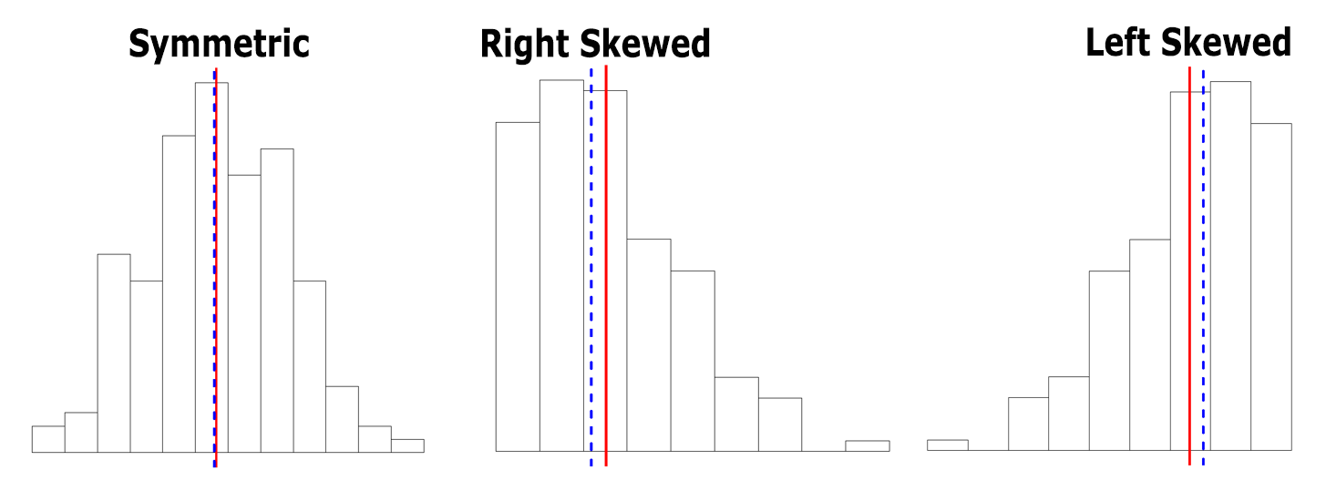
We can tell from the figures:
- For the right-skewed distribution (longer tail on the right-hand side), mean > median because the observations on the right tail drag the mean to the right.
- For the symmetric distribution, mean = median. Both divide the distribution into two parts with roughly equal number of observations.
- For the distribution that is skewed to the left (longer tail on the left-hand side), mean < median because the observations on the left tail drag the mean to the left.
Summary of the Centre
Here are some guidelines for choosing the proper measure to describe the centre of a distribution:
- Use the median when the distribution is extremely skewed or outliers exist.
- Use the mean when the distribution is symmetric and there are no outliers.
- For qualitative/categorical data, we can only use the mode to describe the center.
- For quantitative data, the mode can also be computed. However, it is not as informative as the median or the mean.
