1.4 Organizing Data
Next, we focus on presenting and summarizing data using different tables and figures.
Given a set of data, how can you present the data? It is essential to plot the data before conducting any data analysis. The definition of descriptive statistics tells us we can use tables and graphs to present the data. Different tables and graphs are used to describe the two different types of data—qualitative and quantitative. Let us start with qualitative variables, then continuous and then discrete variables.
1.4.1 Organizing Qualitative Data
Numerically, we can use frequency or relative frequency tables to summarize qualitative/categorical data. Graphically, we can use pie charts or bar charts.
The distribution of a qualitative variable is given in a frequency (relative frequency) table. For example, the students were asked, "How you came to school today?" Fifty-three students answered by car, 136 by public transportation, nine by bicycle, 74 by walking, and one by other means. The results are summarized in the following table.
Table 1.3: Frequency and Relative Frequency Table of "Transportation"
| Transportation | Frequency | Relative Frequency | Percentage |
| Car | 53 | 53/273 = 0.1941 | 19.41% |
| Public | 136 | 136/273 = 0.4982 | 49.82% |
| Bicycle | 9 | 9/273 = 0.0330 | 3.30% |
| Walking | 74 | 74/273 = 0.2710 | 27.10% |
| Other | 1 | 1/273 = 0.0037 | 0.36% |
| Total | 273 | 1.000 | 100% |
- The first column gives all possible outcomes of the variable, which are called categories.
- The second column gives the number of observations falling into each category; we call this number the frequency of that category. For example, the frequency of taking public transit is 136.
- The third column gives the relative frequency, which is calculated as:
[latex]\text{relative frequency} = \frac{\text{frequency}}{\text{total}}.[/latex]
For example, the relative frequency of taking public transit is 0.4982, which means 49.82% of the students came to school by public transit. Note that the relative frequencies always add up to 1 across all the categories.
- The fourth column gives the percentage, which is calculated as [latex]\text{percentage=relative frequency}\times 100[/latex].
Based on the (relative) frequency table, we can draw a bar chart or a pie chart to summarize the data.
- A bar chart represents each category with a bar whose height equals each category's relative frequency or frequency. The bars are plotted next to each other without touching each other. One bar for one category.
- A pie chart is a disc divided into wedge-shaped pieces whose areas are proportional to the relative frequencies. One slice for one category, the angle of each slice = relative frequency x 360°.
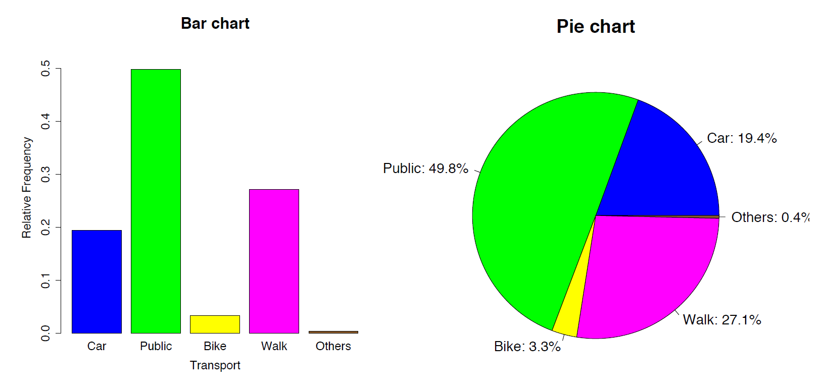
If the bar chart and pie chart are generated based on counts, the charts won't change except for the scale—the relative frequency in the bar chart and the percentage in the pie chart will be replaced by counts or frequency.
Suppose that another qualitative variable recorded in the study was "gender.", we can also present the data characterized by two qualitative variables in what is referred to as a contingency table. Below is the contingency table with the two qualitative variables, gender and transport:
Table 1.4: Contingency Table of "Gender" and "Transportation"
| Car | Public | Bicycle | Walking | Others | Total | |
|---|---|---|---|---|---|---|
| Female | 25 | 80 | 5 | 38 | 0 | 148 |
| Male | 28 | 56 | 4 | 36 | 1 | 125 |
| Total | 53 | 136 | 9 | 74 | 1 | 273 |
The variable "Gender" is called the row variable (shown in red font in the table) and "Transportation" is the column variable (shown in blue font in the table). The totals "148" and "125" (in red) are called row totals (sum across transportation for each category of "gender"). The totals "53," "136," "9," "74," "1" are called column totals (sum across gender for each category of "Transportation"), and "273" is the grand total. Those 10 numbers in bold are called cells.
One interesting question is whether the pattern of transportation among females is the same as that among males. We can compare the relative frequencies of all the categories for females with their counterparts among males. There are 148 female students and 125 male students in total; therefore, the relative frequencies of the five categories for females are 25/148, 80/148, 5/148, 38/148, 0/148 as compared to 28/125, 56/125, 4/125, 36/125, 1/125 for males.
The distributions of "transportation" for females and males can be compared graphically using a side-by-side pie chart and a side-by-side bar chart.
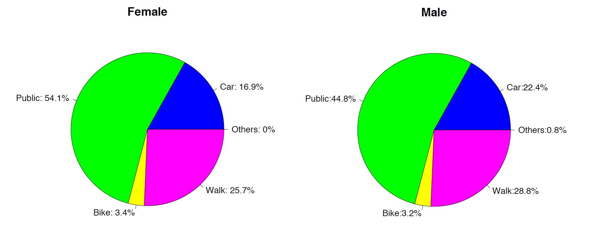
The side-by-side pie chart shows that the patterns in transportation among females and male are very similar, since the two pie charts are almost identical. The side-by-side bar chart based on the relative frequency gives the same conclusion: the distributions of "transportation" for female and male are very similar, which implies there is no significant difference between female and male in the way they come to school.
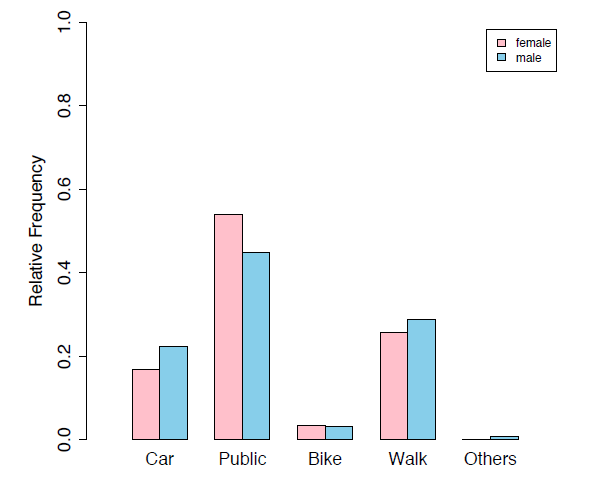

When we compare the distributions of two different groups using a side-by-side bar chart, we should use the relative frequency as the y-axis. Using frequency as the y-axis and comparing the frequencies alone, without taking into account the total of each group, can be misleading.
1.4.2 Organizing Quantitative Discrete Data
We are able to list all possible values for a quantitative discrete variable; therefore, for a quantitative discrete variable with only a few different values, we can describe it using tools similar to those for qualitative variables, i.e., a (relative) frequency table and histogram.
A histogram is somewhat similar to a bar chart. The x-axis shows the value of the variable of interest and the y-axis displays either frequencies or relative frequencies. Histograms can be used to describe both quantitative discrete and quantitative continuous variables. For a continuous variable, we cut the range of the variable into subintervals of equal width and draw one rectangle for each subinterval; the height of the rectangle is the number of observations falling into the corresponding subinterval. For a discrete variable with a small number of possible values, we can draw a rectangle with equal width for each value, the height of each rectangle is either the frequency or relative frequency.
Example: Organizing Quantitative Discrete Variables
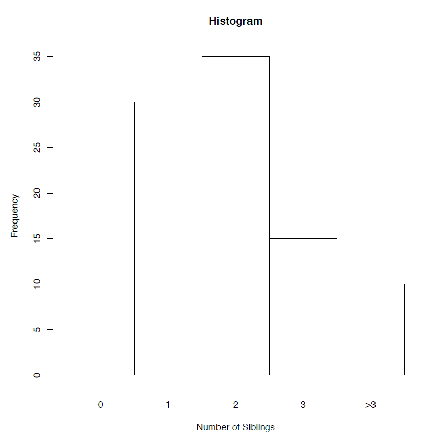
There are 100 students in a class; ten have no siblings, thirty have one sibling, thirty-five have two siblings, fifteen have three siblings, and ten have more than three siblings.
We can use a (relative) frequency table and a histogram to summarize the data.
Table 1.5: Frequency and Relative Frequency Table of "# of Siblings"
| Total | 100 | 1.00 |
| # of Siblings | Frequency | Relative Frequency |
| 0 | 10 | 0.10 |
| 1 | 30 | 0.30 |
| 2 | 35 | 0.35 |
| 3 | 15 | 0.15 |
| >3 | 10 | 0.10 |
Difference between a bar chart and a histogram:
- The bars of a bar chart do not touch one another. Since there is often no inherent ordering among the categories, the order among the bars is usually irrelevant (i.e., bars can be switched without affecting the usefulness of the graph).
- The adjacent bars of a histogram do touch one another. Since there is ordering among numbers, that ordering is to be preserved among the bars of a histogram. That is, the first bar corresponds to the smallest value (or the interval of the smallest values), the second bar corresponds to the second smallest value (or the interval of the second smallest values), and so on.
1.4.3 Organizing Quantitative Continuous Data
Example: Organizing Quantitative Continuous Variables
Here are the 50 grades for an exam:
| 68 | 72 | 59 | 56 | 60 | 40 | 55 | 68 | 76 | 75 |
| 46 | 59 | 37 | 54 | 83 | 85 | 29 | 55 | 56 | 42 |
| 50 | 49 | 65 | 68 | 61 | 53 | 55 | 92 | 68 | 48 |
| 79 | 51 | 24 | 57 | 48 | 71 | 90 | 81 | 34 | 60 |
| 47 | 39 | 65 | 74 | 49 | 52 | 59 | 9 | 62 | 37 |
How to present and summarize these data?
Grouping Table and Histogram
Recall that all values of a discrete variable can be listed. However, this is not the case for a continuous variable: we cannot list all possible values for a continuous variable. For example, even though the above 50 grades are all reported as whole numbers, there is no reason why a grade couldn’t contain a decimal, such as [latex]46.5[/latex], or [latex]66. \bar{6}[/latex]. For this reason, it is most appropriate to view the grade variable as a continuous variable. Even though we cannot list all possible values of a continuous variable, we can cut the range of a continuous variable into subintervals of equal width and use histograms to summarize quantitative continuous data. The range of grade is [0, 100], a convenient and neat cut is by intervals with width of 10 or 20. If we cut by intervals of 10, the resulting grouping data and histogram are as follows:
Table 1.6: Grouping Table of Grade for Histogram
| Total | 50 | 1.00 |
| Interval | Frequency | Relative Frequency |
| [0, 10) | 1 | 1/50=0.02 |
| [10, 20) | 0 | 0/50=0.00 |
| [20, 30) | 2 | 2/50=0.04 |
| [30, 40) | 4 | 4/50=0.08 |
| [40, 50) | 8 | 8/50=0.16 |
| [50, 60) | 14 | 14/50=0.28 |
| [60, 70) | 10 | 10/50=0.20 |
| [70, 80) | 6 | 6/50=0.12 |
| [80, 90) | 3 | 3/50=0.06 |
| [90, 100] | 2 | 2/50=0.04 |
Please note that we still need to keep those intervals that have no observations. For example, the interval [10, 20) includes 10 but excludes 20, and has no observations. We need to keep this interval when we draw a histogram for the data.

- A common question when drawing histograms is whether to use [, ) or (, ] intervals. Please note that different software may follow different rules. It is important to consistently follow the same rule for all intervals in your histogram.
- Another common question is how many bins is proper. A rule of thumb is the square root of the number of observations. For the grade example, since [latex]n=50[/latex] and [latex]\sqrt{n}=\sqrt{50}=7.07[/latex]. The range of grade is [0, 100], to create convenient cuts, we can divide the range either into 10 subintervals with equal length, i.e., [latex][0, 10), [10, 20), \cdots, [90, 100][/latex] or 5 subintervals with equal width, i.e., [latex][0, 20), [20, 40), \cdots, [80, 100][/latex].
- Note that histograms with different number of bins might appear very different. When investigating the shape of the distribution of a variable using a histogram, it is always better to draw a boxplot and normal Q-Q plot as well. Boxplot and normal Q-Q plot will be covered in sections 2.4 and 5.6 respectively.
Stem-and-Leaf Diagram
Another way to present quantitative data is a stem-and-leaf diagram. To construct a stem-and-leaf diagram:
- Think of each observation consisting of a stem (all but the rightmost digit) and a leaf (the rightmost digit, a single digit).
- Draw a vertical line, write the stems from the smallest to the largest in a vertical column to the left of the vertical line.
- Write each leaf to the right of the vertical line in the same row as its corresponding stem.
- Arrange the leaves in each row from the smallest to the largest.
- Indicate the decimal place of the data if applicable.
Let’s return to the grades data:
| 68 | 72 | 59 | 56 | 60 | 40 | 55 | 68 | 76 | 75 |
| 46 | 59 | 37 | 54 | 83 | 85 | 29 | 55 | 56 | 42 |
| 50 | 49 | 65 | 68 | 61 | 53 | 55 | 92 | 68 | 48 |
| 79 | 51 | 24 | 57 | 48 | 71 | 90 | 81 | 34 | 60 |
| 47 | 39 | 65 | 74 | 49 | 52 | 59 | 9 | 62 | 37 |
We can group the grades by the first digits (in intervals of 10) as follows,
Table 1.7: Working Table for Stem-and-Leaf Diagram
| Interval | Data |
| [0, 10) | 9 |
| [10, 20) | |
| [20, 30) | 24, 29 |
| [30, 40) | 34, 37, 37, 39 |
| [40, 50) | 40, 42, 46, 47, 48, 48, 49, 49, |
| [50, 60) | 50, 51, 52, 53, 54, 55, 55, 55,56, 56, 57, 59, 59, 59 |
| [60, 70) | 60, 60, 61, 62, 65, 65, 68, 68, 68, 68, 68 |
| [70, 80) | 71, 72, 74, 75, 76, 79 |
| [80, 90) | 81, 83, 85 |
| [90, 100] | 90, 92 |
If we take apart the grades and mark the first digit at left side of the line and the second digit at the right side of the line, it becomes a stem-leaf diagram:
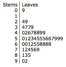
Decimal place: 9|0 = 90
Figure 1.7: Stem-and-Leaf Diagram of Grade [Image Description (See Appendix D Figure 1.7)]
The part "Decimal place: 9|0 = 90" indicates that the decimal point is one digit to the right of the vertical line.
Some other useful guidelines of the stem-and-leaf diagram are as follows:
|
 |
Example
Let's consider two data sets. Data set I: 3600, 1500, 6900 and Data set II: 0.36, 0.15, 0.69. It is not a good idea to draw the stem-and-leaf diagram based on the original data sets. Take Data set I for example, all three numbers have a leaf of 0 (the right most digit) and there are many stems without leaves between 150 and 360. Therefore, we divide the numbers by 100 and transform the numbers to 36, 15 69 to draw a stem-and-leaf diagram. Finally, we indicate the decimal point by putting 6|9=6900 at the bottom of the graph. Similarly, we multiply all three numbers 0.36, 0.15, 0.69 by 100 to create a new data set: 36, 15, 69 and then draw a stem-and-leaf diagram.
These two data sets have the same resulting stem-and-leaf diagram as the data set 36, 15, and 69. However, the decimal point is 3 digits to the right of the vertical line for Date set I, i.e., we should indicate 6|9=6900; the decimal point is one digit to the left of the vertical line for Date set II, i.e., 6|9=0.69.
Stem-and-Leaf Diagram for Data set 1: 3600, 1500, 6900
Decimal 6|9=6900 |
Stem-and-Leaf Diagram for Data set 2: 0.36, 0.15, 0.69
Decimal 6|9=0.69 |
