5.2 Normal Density Curve

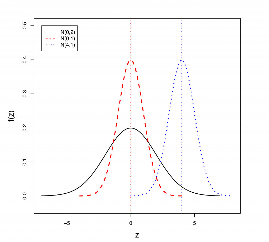
The normal density curve characterizes the normal distribution, which is the most widely used probability distribution for continuous variables. The normal distribution is symmetric and bell-shaped (for this reason it is often referred to as the “bell curve”). The normal density function has two parameters: the mean [latex]\mu[/latex] and the standard deviation [latex]\sigma[/latex]. The parameter [latex]\mu[/latex] controls the centre (location) of the distribution and [latex]\sigma[/latex] controls the shape of the distribution. When [latex]\sigma[/latex] is larger, the curve appears shorter and fatter; when [latex]\sigma[/latex] is smaller, the curve appears taller and slimmer.

Figure 5.2 shows three normal density curves–[latex]N(0, 2), N(0, 1)[/latex] and [latex]N(4, 1)[/latex]. [latex]N(0,1)[/latex] and [latex]N(4, 1)[/latex] have the same standard deviation; therefore, they have the same shape; if you shift the location of [latex]N(0, 1)[/latex] to the right by 4, the two distributions are exactly the same. [latex]N(0,1)[/latex] and [latex]N(0, 2)[/latex] have the same mean; therefore, they center at the same location. [latex]N(0, 2)[/latex] has a larger standard deviation; therefore, the density curve is shorter and fatter.

If a random variable [latex]X[/latex] follows a normal distribution with mean [latex]\mu[/latex] and standard deviation [latex]\sigma[/latex], we write [latex]X \sim N(\mu, \sigma)[/latex]. The probability density function of a normal random variable [latex]X[/latex] is given by:

[latex]f(x) = \frac{1}{\sqrt{2 \pi} \sigma} e^{-\frac{(x- \mu)^2}{2\sigma^2}}, -\infty < x < \infty  \text { with } \pi \approx 3.142 \text { and } e \approx 2.718[/latex].

The normal density curve has the following properties:

Key Facts: Properties of a Normal Density Curve

• The curve extends from negative infinity [latex](-\infty)[/latex] to positive infinity [latex](\infty)[/latex], i.e., the entire real line.
• The total area under the curve is 1. This is a common property for all density curves.
• The curve is bell-shaped, unimodal, and symmetric at the mean [latex]\mu[/latex].
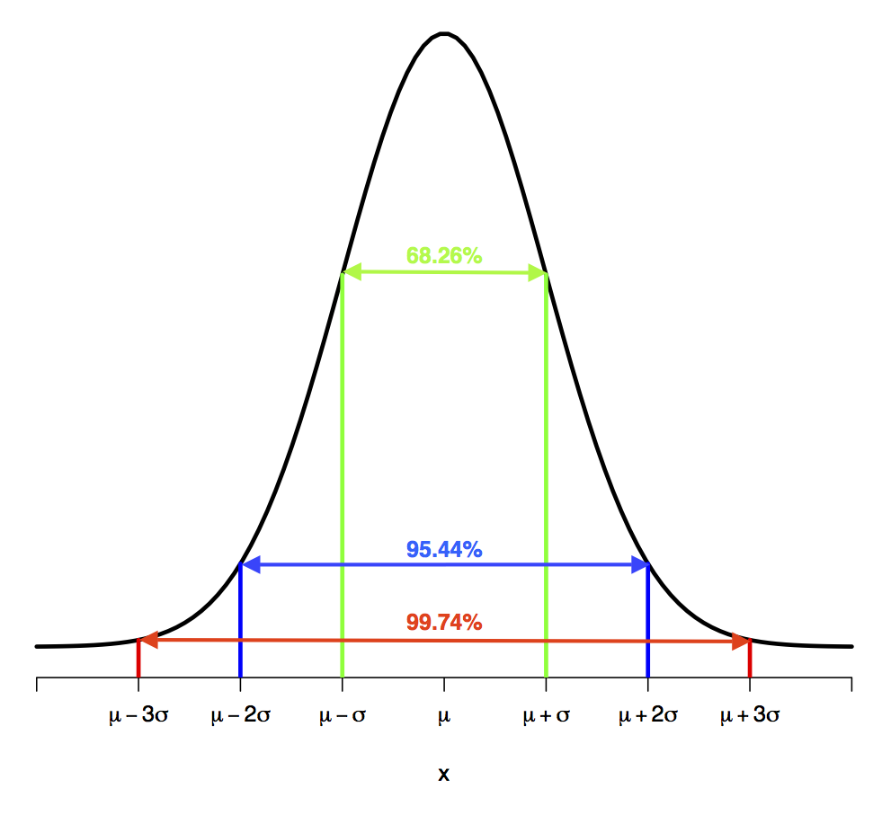
• Empirical rule (68.3-95.4-99.7 rule) for a normal curve:

1. 1. 68.26% of the observations are within the interval [latex][\mu - \sigma, \mu + \sigma][/latex] (one standard deviation to either side of the mean), i.e., [latex]P(\mu - \sigma \leq X \leq \mu + \sigma) = 0.6826.[/latex]
   2. 95.44% of the observations are within the interval [latex][\mu - 2\sigma, \mu + 2\sigma][/latex] (two standard deviations to either side of the mean), i.e., [latex]P(\mu - 2\sigma \leq X \leq \mu + 2\sigma) = 0.9544.[/latex]
   3. 99.74% of the observations are within the interval [latex][\mu - 3\sigma, \mu + 3\sigma][/latex] (three standard deviations to either side of the mean), i.e., [latex]P(\mu - 3\sigma \leq X \leq \mu + 3\sigma) = 0.9974.[/latex]