3.7 Tree Diagrams
A tree diagram is a helpful tool, used to display a sequence of events and their conditional probabilities. Each branch of the tree corresponds to one possible outcome in the sequence of the events; and the probability of the outcome equals the product of all subsequent probabilities on the branch. Tree diagrams provide a useful illustration of the general multiplication rule.
Example: Tree Diagram
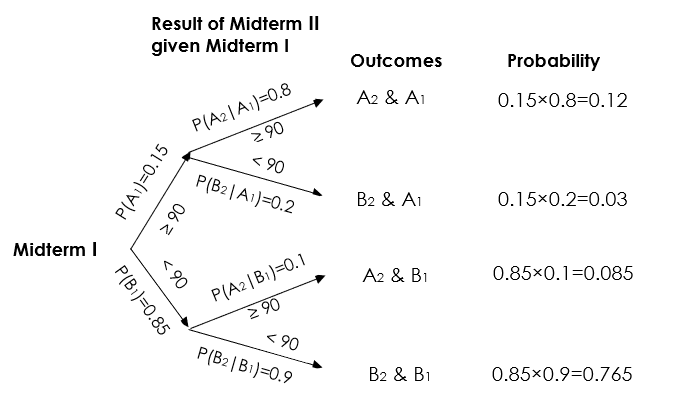
Suppose we have two midterms, the probability that you get at least 90 in Midterm I is 0.15. If you get at least 90 in Midterm I, then the probability that you get at least 90 in Midterm II is 0.8; if you do not receive at least 90 in Midterm I, the probability that you will receive at least 90 in Midterm II is 0.1. We could use a tree diagram to present the probabilities.
Let’s define the events:
[latex]A_1[/latex] = obtaining at least 90 in Midterm I, [latex]B_1[/latex] = obtaining below 90 in Midterm I
[latex]A_2[/latex] = obtaining at least 90 in Midterm II, [latex]B_2[/latex] = obtaining below 90 in Midterm II
We can summarize the information given in the question using probability notations.
[latex]P(A_1) = 0.15; \quad P(B_1) = 1-P(A_1)=1-0.15=0.85;[/latex]
[latex]P(A_2|A_1)=0.8; \quad P(A_2|B_1) = 0.1;[/latex]
[latex]P(B_2|A_1) =1-0.8= 0.2; \quad P(B_2|B_1) = 1-0.1 = 0.9 .[/latex]
Then the tree diagram is presented as follows:
- Find the probability that a student obtained at least 90 in both midterms.
[latex]P(A_1 \: \& \: A_2)= P(A_1) \times P(A_2 |A_1)=0.15 \times 0.8=0.12.[/latex]
Note that due to the multiplication rule, the probability of each outcome equals the product of all subsequent probabilities on the corresponding branch.
- Find the probability that a student obtained at least 90 in exactly one midterm.
[latex]\begin{align*} P(A_1 \: \& \: B_2 \text{ or } B_1 \: \& \: A_1) &= P(A_1 \: \& \: B_2) + P(B_1 \: \& \: A_2)\\ &= P(A_1) \times P(B_2|A_1) + P(B_1) \times P(A_2|B_1)\\ &= 0.15 \times 0.2 + 0.85 \times 0.1 = 0.03 + 0.085= 0.115. \end{align*}[/latex] - Find the probability that a student obtained at least 90 in at least one of the midterms.
[latex]\begin{align*} P(A_1 \: \& \: A_2 \text{ or } A_1 \: \& \: B_2 \text{ or } A_2 \: \& \: B_1)& = 1 - P(B_1 \: \& \: B_2) = 1- P(B_1) \times P(B_2|B_1)\\ &= 1- 0.85 \times 0.9 = 1 - 0.765 = 0.235, \end{align*}[/latex]
OR
[latex]\begin{align*} P(A_1 \: \& \: A_2 \text{ or } A_1 \: \& \: B_2 \text{ or } B_1 \: \& \: A_2)&=P(A_1 \: \& \: A_2)+P(A_1 \: \& \: B_2)+ P(B_1 \: \& \: A_2)\\ &=0.12+0.03+0.085=0.235. \end{align*}[/latex]
Exercise: Tree Diagram
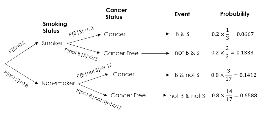
It is believed that there is an association between breast cancer and smoking. The following table summarizes results of an observational study of 200 females who are classified by their disease status and smoking status.
| Smoker (S) | Non-smoker (not S) | Total | |
|---|---|---|---|
| Breast Cancer (B) | 10 (B & S) | 30 (B & not S) | 40 (B) |
| Cancer Free (not B) | 20 (not B & S) | 140 (not B & not S) | 160 (not B) |
| Total | 30 (S) | 170 (not S) | 200 |
Represent the information given in the contingency table above in a tree diagram, branching first on smoking status and then on breast cancer status.