8.5 Hypothesis Tests for One Population Mean μ
Recall that there are two different procedures used to construct confidence intervals for one population mean [latex]\mu[/latex]: the one-sample Z-interval (used when the population standard deviation [latex]\sigma[/latex] is known) and the one-sample t-interval (used when [latex]\sigma[/latex] is unknown). In a similar vein, there are two different procedures for hypothesis tests for one population mean: the one-sample Z-test is used when [latex]\sigma[/latex] is known and the one-sample t-test is used when [latex]\sigma[/latex] is unknown.
8.5.1 One-Sample Z-Test When σ is Known
Assumptions:
- A simple random sample (SRS)
- Normal population or large sample size ([latex]n \geq 30[/latex])
- The population standard deviation [latex]\sigma[/latex] is known
Steps:
- Set up the hypotheses (one of the following three pairs):
Two tailed Right tailed Left tailed [latex]H_0: \mu = \mu_0[/latex] [latex]H_0: \mu \leq \mu_0[/latex] [latex]H_0: \mu \geq \mu_0[/latex] [latex]H_a: \mu \neq \mu_0[/latex] [latex]H_a: \mu > \mu_0[/latex] [latex]H_a: \mu < \mu_0[/latex] - State the significance level [latex]\alpha[/latex].
- Compute the value of the test statistic: [latex]z_o = \frac{\bar{x} - \mu_0}{\sigma / \sqrt{n}}[/latex].
- Find the P-value or rejection region.
Two tailed Right tailed Left tailed [latex]H_0[/latex] [latex]H_0: \mu = \mu_0[/latex] [latex]H_0: \mu \leq \mu_0[/latex] [latex]H_0: \mu \geq \mu_0[/latex] [latex]H_a[/latex] [latex]H_a: \mu \neq \mu_0[/latex] [latex]H_a: \mu >\mu_0[/latex] [latex]H_a: \mu < \mu_0[/latex] P-value [latex]2P(Z \geq |z_o|)[/latex] [latex]P(Z \geq z_o)[/latex] [latex]P(Z \leq z_o)[/latex] Rejection region [latex]Z \geq z_{\alpha / 2}[/latex] or [latex]Z \leq -z_{\alpha / 2}[/latex] [latex]Z \geq z_{\alpha}[/latex] [latex]Z \leq -z_{\alpha}[/latex] - Reject the null [latex]H_0[/latex] if P-value [latex]\leq \alpha[/latex] or [latex]z_o[/latex] falls in the rejection region.
- Conclusion.
Example: One-Sample Z Test
One-Sample Z Test
A machine fills beer into bottles whose volume is supposed to be 341 ml, but the exact amount varies from bottle to bottle. We randomly picked 100 bottles and obtained the sample mean volume of 339 ml. Assume the population standard deviation [latex]\sigma = 5[/latex] ml. Test at the 5% significance level whether the machine is NOT working properly.
Check the assumptions:
- We have a simple random sample (SRS).
- We do not know whether the population is normal or not, but the sample size is large with [latex]n = 100 \geq 30[/latex].
- [latex]\sigma = 5[/latex] ml is known.
Steps:
- Set up the hypotheses: [latex]H_0: \mu = 341[/latex] ml versus [latex]H_a: \mu \neq 341[/latex] ml.
This is a two-tailed test. If the machine works properly, the population mean volume [latex]\mu = 341[/latex] ml.
- The significance level is [latex]\alpha = 0.05[/latex].
- Compute the value of the test statistic:
[latex]z_o = \frac{\bar{x} - \mu_0}{\sigma / \sqrt{n}} = \frac{339 - 341}{5 / \sqrt{100}} = \frac{-2}{0.5} = -4.[/latex]
- Find the P-value. For a two-tailed test with the observed test statistic [latex]z_o = – 4[/latex].


P-value = [latex]2P(Z \leq -4) \approx 2 \times 0 = 0.[/latex]
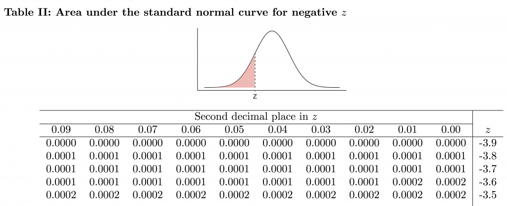
[Image Description (See Appendix D Example 8.1)] - Decision: Since the P-value [latex]\approx 0 \leq 0.05(\alpha)[/latex], reject the null hypothesis [latex]H_0[/latex].
- Conclusion: At the 5% significance level, the data provide sufficient evidence that the machine is NOT working properly.

If using the critical value approach, steps 1-3 are the same, steps 4-6 become:
- Rejection region:
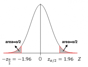
[Image Description (See Appendix D Example 8.2)] [latex]\alpha = 0.05, z_{\alpha / 2} = z_{0.05 / 2} = z_{0.025} = 1.96.[/latex] For a two-tailed test, the critical values are -1.96 and 1.96. The rejection region is either greater than 1.96 or smaller than -1.96.
- Decision: Since the observed value [latex]z_o= -4 <-1.96[/latex] falls in the rejection region, we reject the null hypothesis [latex]H_0[/latex].
- Conclusion: At the 5% significance level, the data provide sufficient evidence that the machine is NOT working properly.

P-value approach is preferred for the following reasons:
- It is more professional. P-value is required to be reported for all hypothesis tests in academia.
- The P-value approach provides more information: it not only tells whether we should reject the null or not but also shows how strong the evidence is. However, the critical value approach only tells us whether we should reject the null or not.
- The computer output only provides the P-value; no critical value is provided.
8.5.2 One-Sample t-Test When σ is Unknown
Assumptions:
- A simple random sample (SRS)
- Normal population or large sample size ([latex]n \geq 30[/latex])
- The population standard deviation [latex]\sigma[/latex] is unknown
Steps:
- Set up the hypotheses:
Two tailed Right tailed Left tailed [latex]H_0: \mu = \mu_0[/latex] [latex]H_0: \mu \leq \mu_0[/latex] [latex]H_0: \mu \geq \mu_0[/latex] [latex]H_a: \mu \neq \mu_0[/latex] [latex]H_a: \mu \: \gt \: \mu_0[/latex] [latex]H_a: \mu < \mu_0[/latex] - State the significance level [latex]\alpha[/latex].
- Compute the value of the test statistic: [latex]t_o = \frac{\bar{x} - \mu_0}{s / \sqrt{n}}[/latex] with a degree of freedom [latex]df = n-1[/latex].
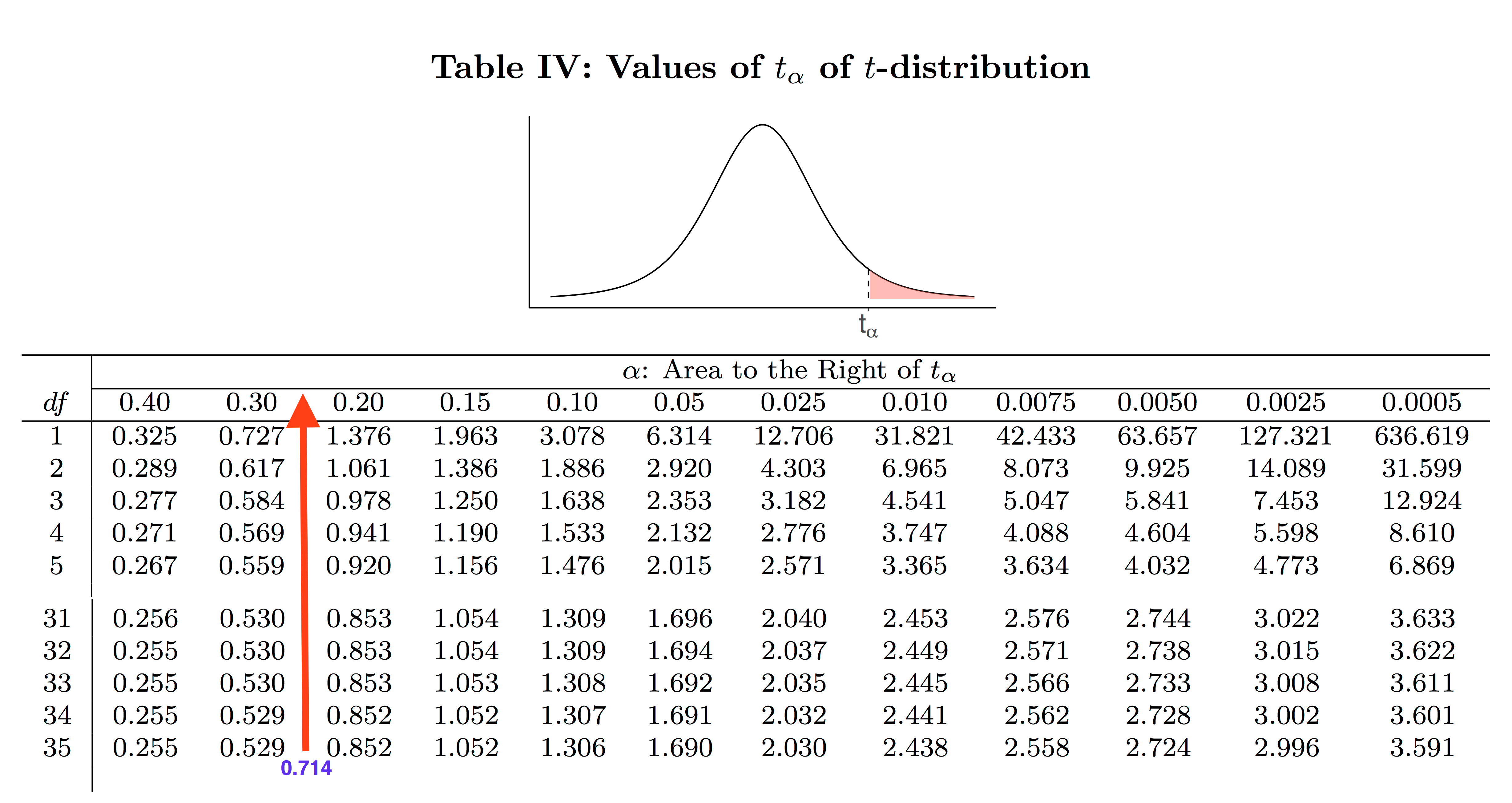
- Use the t score table (Table IV) to find the P-value or rejection region.
Two tailed Right tailed Left tailed [latex]H_0[/latex] [latex]H_0: \mu = \mu_0[/latex] [latex]H_0: \mu \leq \mu_0[/latex] [latex]H_0: \mu \geq \mu_0[/latex] [latex]H_a[/latex] [latex]H_a: \mu \neq \mu_0[/latex] [latex]H_a: \mu \: \gt \: \mu_0[/latex] [latex]H_a: \mu < \mu_0[/latex] P-value [latex]2P(t \geq |t_o|)[/latex] [latex]P(t \geq t_o)[/latex] [latex]P(t \leq t_o)[/latex] Rejection region [latex]t \geq t_{\alpha/2}[/latex] or [latex]t \leq -t_{\alpha/2}[/latex] [latex]t \geq t_{\alpha}[/latex] [latex]t \leq -t_{\alpha}[/latex] Note: Unlike the p-value of a one-sample [latex]Z[/latex] test when [latex]\sigma[/latex] is known, in general, only a range of values rather than an exact number will be obtained for a one-sample [latex]t[/latex] test using Table IV. An exact p-value will be obtained only when the observed test statistic is one of those twelve t-scores given in the table for a given degree of freedom.
- Reject the null [latex]H_0[/latex] if P-value [latex]\leq \alpha[/latex] or [latex]t_o[/latex] falls in the rejection region.
- Conclusion.
Example: One-Sample t Test
A computer company claims that the average lifetime of its laptop is about 4 years. A simple random sample of 36 laptops yields an average lifetime of 3.5 years with a sample standard deviation of 4.2 years. Test at the 1% significance level whether the mean lifetime of this brand of laptops is less than 4 years.
Check the assumptions:
- We have a simple random sample (SRS).
- We do not know whether the population is normal or not, but the sample size is large with [latex]n = 36 \geq 30[/latex].
- [latex]\sigma[/latex] is unknown and estimated by [latex]s = 4.2[/latex].
Steps:
- Set up the hypotheses: [latex]H_0: \mu \geq 4[/latex] years versus [latex]H_a: \mu < 4[/latex] years.
- The significance level is [latex]\alpha = 0.01[/latex].
- Compute the value of the test statistic:
[latex]t_o = \frac{\bar{x} - \mu_0}{s / \sqrt{n}} = \frac{3.5 - 4}{4.2 / \sqrt{36}} = \frac{-0.5}{0.7} = -0.714[/latex] with [latex]df = n -1 = 36 -1 = 35[/latex]. - Find the P-value. For a left-tailed test, the P-value is the area to the left of the observed test statistic [latex]t_o[/latex] because the alternative [latex]H_a[/latex] is "<".
P-value= [latex]P(t \leq t_o)[/latex] [latex]= P(t \leq -0.714)[/latex] [latex]= P(t \geq 0.714) \: \gt \: 0.2.[/latex] To be more precisely, [latex]0.2<\mbox{p-value}<0.3.[/latex]
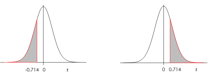
[Image Description (See Appendix D Example 8.3)] - Decision: Since the P-value [latex]\: \gt \: 0.2 \: \gt \: 0.01(\alpha)[/latex], we can not reject the null [latex]H_0[/latex].
- Conclusion: At the 1% significance level, we do not have sufficient evidence that the mean lifetime of this brand of laptops is less than 4 years.
If we use the critical value approach, steps 1-3 are the same, and steps 4-6 become:
- Rejection region
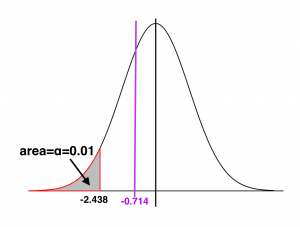
[Image Description (See Appendix D Example 8.4)] [latex]df = n-1 = 36 -1 =35[/latex], [latex]\alpha = 0.01, t_{\alpha} = t_{0.01} = 2.438[/latex]
For a left-tailed test, the critical value is [latex]-t_{\alpha} = -t_{0.01} = -2.438[/latex].
- Decision: Since the observed value [latex]t_o = -0.714 \: \gt \: - 2.438[/latex] falls in the non-rejection region, we can not reject the null hypothesis [latex]H_0[/latex].
- Conclusion: At the 1% significance level, the data do not provide sufficient evidence that the mean lifetime of this brand of laptops is less than 4 years.

Exercise: P-value for One sample t-Test
Use the same setting of the previous example (one-sample t-test with df = 35) to find the P-values of the following hypothesis tests.
- [latex]H_0: \mu = 4 \text{ years versus } H_a: \mu \neq 4 \text{ years}[/latex], with the observed test statistic [latex]t_o = 1.5[/latex].
- [latex]H_0: \mu \geq 4 \text{ years versus } H_a: \mu < 4 \text{ years}[/latex], with the observed test statistic [latex]t_o=-2.5[/latex].
- [latex]H_0: \mu \leq 4 \text{ years versus } H_a: \mu \: \gt \: 4 \text{ years}[/latex], with the observed test statistic [latex]t_o = 3.5[/latex].
Show/Hide Answer
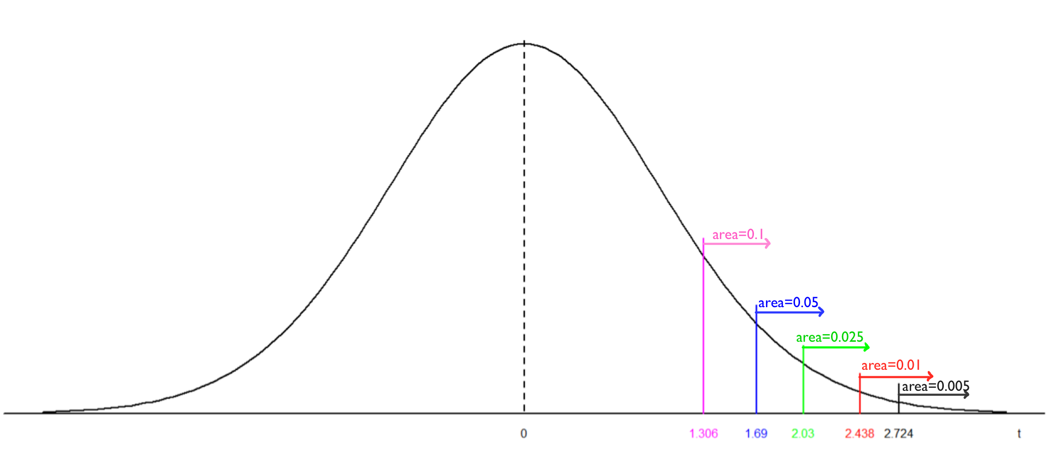
- For a two-tailed test, the P-value is twice the area to the right of the absolute value of the observed test statistic [latex]t_o[/latex]. Note that the probability is the area under the density curve of the t-distribution with 35 degrees of freedom.[latex]P[/latex]-value=[latex]2P(t\ge |t_o|)=2P(t\ge 1.5)[/latex]. Since [latex]1.306 (t_{0.1})<1.5<1.690 (t_{0.05})[/latex], we have [latex]0.05 \lt P(t\ge 1.5) \lt 0.1 \Longrightarrow 2\times 0.05 \lt 2 P(t\ge 1.5) \lt 2\times 0.1[/latex] [latex]\Longrightarrow 0.1 \lt \mbox{P-value} \lt 0.2.[/latex] If use R commander, [latex]2 P(t\ge 1.5)=2\times 0.07129092=0.1425818[/latex].
- For a left-tailed test, the P-value is the area to the left of the observed test statistic [latex]t_o[/latex]. [latex]P[/latex]-value=[latex]P(t \le t_o )=P(t \le -2.5)=P(t \ge 2.5)[/latex]. Since[latex]2.438(t_{0.01})<2.5<2.558(t_{0.0075}) \Longrightarrow 0.0075<\mbox{P-value}< 0.01.[/latex] If use R commander, [latex]P(t \ge 2.5)=0.008627872[/latex].
- For a right-tailed test, the P-value is the area to the right of the observed test statistic [latex]t_o[/latex].[latex]P[/latex]-value=[latex]P(t\ge t_o )=P(t\ge 3.5)[/latex]. Since[latex](t_{0.0025})2.996<3.5<3.591(t_{0.0005}) \Longrightarrow 0.0005<\mbox{P-value}<0.0025.[/latex] If use R commander, [latex]P(t \ge 3.5)=0.0006444197[/latex].
Exercise: One-sample t-Test
The number of cell phone users has increased dramatically since 1997. Suppose the mean local monthly bill was $50 for cell phone users in the United States in 2006. A simple random sample of 50 cell phone users was obtained in 2019, and the sample mean local monthly bill was [latex]\bar{x} = 55[/latex] with a sample standard deviation [latex]s = $25[/latex].
- At the 5% significance level, do the data provide sufficient evidence to conclude that the mean local monthly bill for cell phone users in 2019 has changed from the 2006 mean of $50?
- Obtain a 95% confidence interval for the 2019 mean local monthly bill for all cell phone users. Interpret the confidence interval.
- Are the results in parts (a) and (b) consistent with each other? Explain why.
Show/Hide Answer
- Check the assumptions:
- We have a simple random sample (SRS).
- We do not know whether the population is normal or not since we do not have the data, but the sample size is large with [latex]n = 50 \geq 30[/latex].
- [latex]\sigma[/latex] is unknown and estimated by [latex]s = $25[/latex].
Steps:
- Set up the hypotheses: [latex]H_0: \mu = 50[/latex] versus [latex]H_a: \mu \neq 50[/latex].
- The significance level is [latex]\alpha = 0.05[/latex].
- Compute the value of the test statistic: [latex]t_o = \frac{\bar{x} - \mu_0}{s / \sqrt{n}} = \frac{55 - 50}{25 / \sqrt{50}} = 1.414[/latex] with [latex]df = n-1 = 50 -1 = 49[/latex].
- Find the P-value. For a two-tailed test, the P-value is twice the area to the right of the observed test statistic [latex]t_o[/latex].
P-value=[latex]2P(t \geq t_o) = 2P(t \geq 1.414)[/latex]. Since [latex]1.299(t_{0.1}) < 1.414 < 1.677(t_{0.05})[/latex], [latex]2\times 0.05 < \text{P-value} <2\times 0.1 \Longrightarrow 0.1<\text{P-value}<0.2.[/latex] - Decision: Since the P-value [latex]\: \gt \: 0.1>0.05 (\alpha)[/latex], we can not reject the null [latex]H_0[/latex].
- Conclusion: At the 5% significance level, we do not have sufficient evidence that the 2019 mean local monthly bill for cell phone users has changed from the 2006 mean of $50.
- Steps:
- Find [latex]t_{\alpha / 2}[/latex]: [latex]n = 50, df = n-1 = 50-1 =49[/latex].
[latex]1 - \alpha = 0.95 \Longrightarrow \alpha = 0.05 \Longrightarrow \alpha / 2 = 0.025 \Longrightarrow t_{\alpha / 2} = t_{0.025} = 2.010[/latex]. - Interval: [latex]\bar{x} \pm t_{\alpha / 2}\frac{s}{\sqrt{n}} = 55 \pm 2.010 \times \frac{25}{\sqrt{50}} = (47.894, 62.106)[/latex].
Interpretation: We can be 95% confident that the 2019 mean local monthly bill for cell phone users is somewhere between $47.894 and $62.106.
- Find [latex]t_{\alpha / 2}[/latex]: [latex]n = 50, df = n-1 = 50-1 =49[/latex].
- Yes, they are consistent. We cannot reject [latex]H_0: \mu = 50[/latex] and hence can not claim [latex]\mu \neq 50[/latex] in the hypothesis test in part (a). The interval in part (b) contains 50; there is no sufficient evidence that the population mean differs from 50. We cannot reject [latex]H_0: \mu=50[/latex] and claim [latex]\mu \neq 50[/latex]. Therefore, they are consistent.
