13.2 Least-Squares Straight Line
We use a straight line to model the relationship between two quantitative variables y and x: [latex]y = b_0 + b_1 x[/latex]. The interpretations of the terms in the equation are given as follows:
- [latex]x[/latex]: the predictor (independent) variable
- [latex]y[/latex]: the response (dependent) variable
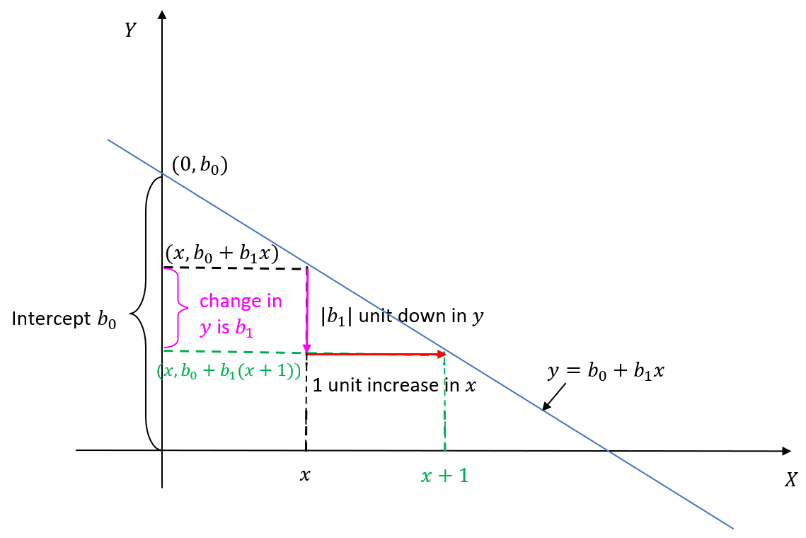
- [latex]b_0[/latex]: the intercept, it is the value of [latex]y[/latex] when [latex]x=0[/latex]
- [latex]b_1[/latex]: the slope of the straight line. It is the change in y when x increases by 1 unit. If [latex]b_1 > 0[/latex], y increases when x increases; if [latex]b_1 < 0[/latex], y decreases when x increases.
The figure below illustrates the meanings of the intercept and the slope of a straight line.
Our first objective is to determine the values of [latex]b_0[/latex] and [latex]b_1[/latex] that characterize the line of best fit: [latex]\hat{y} = b_0 + b_1 x[/latex]. To properly quantify what is meant by "best fit", we introduce some definitions. The fitted values are [latex]\hat{y}_i = b_0 + b_1 x_i[/latex], where [latex]x_i[/latex] is the observed x-value corresponding to [latex]y_i[/latex], the observed y-value, for [latex]i=1, 2, \dots , n[/latex]. Each residual is defined as the difference between the observed [latex]y[/latex] value and the fitted value. That is, the ith residual is:
[latex]e_i = y_i - \hat{y}_i = y_i - (b_0 + b_1 x_i)[/latex].
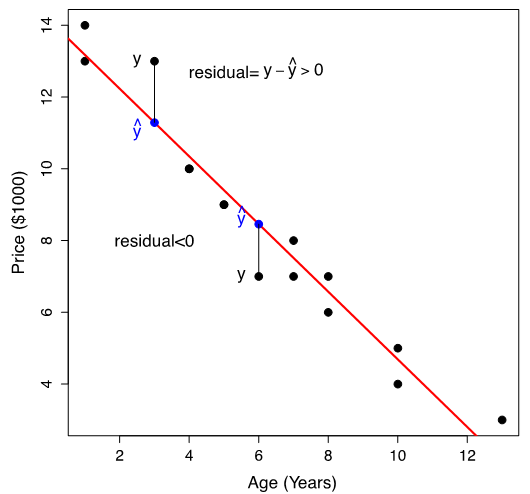
The least-squares regression line is obtained by finding the values of [latex]b_0[/latex] and [latex]b_1[/latex] that minimize the residual sum of squares [latex]SSE = \sum e_i^2 = \sum [ y_i - (b_0 + b_1 x_i) ]^2[/latex]. The figure below illustrates the least-squares regression line as the red line.
Note that:
- Some residuals are positive, and some are negative. Note that [latex]\sum e_i = \sum (y_i - \hat{y}_i) = 0[/latex].
- We want a straight line closest to the data points, i.e., the total distance from the points to the line is minimized.
- We use the square of the residual [latex]e_i^2[/latex] to quantify the distance from the data point [latex]y_i[/latex] to the straight line.
- The total error is the sum of the squared distances from each point to the straight line, i.e., [latex]\sum e_i^2[/latex].
- The straight line yielding the smallest [latex]\sum e_i^2[/latex] is called the least-squares line since it makes the sum of squares of the residuals the smallest.
To find the values of [latex]b_0[/latex] and [latex]b_1[/latex] that minimize the residual sum of squares
[latex]SSE = \sum e_i^2 = \sum [ y_i - (b_0 + b_1 x_i) ]^2[/latex]
is an optimization problem. It can be shown that the solutions are
[latex]\begin{align*}b_1 &= \frac{S_{xy}}{S_{xx}} = \frac{\sum(x_i - \bar{x})(y_i - \bar{y})}{\sum (x_i - \bar{x} )^2} = \frac{\sum x_i y_i - \frac{\left(\sum x_i\right)\left(\sum y_i \right)}{n}}{\sum x_i^2 - \frac{\left(\sum x_i\right)^2}{n}},\\b_0&= \bar{y} - b_1 \bar{x} = \frac{\sum y_i }{n} - b_1 \frac{\sum x_i}{n}.\end{align*}[/latex]
Like ANOVA, the least-squares regression equation can be obtained using software in practice.
Example: Least-Squares Regression Line
Given the summaries of the 15 used cars,
[latex]n = 15, \sum x_i = 92, \sum x_i^2 = 724, \sum y_i = 125, \sum y_i^2 = 1193, \sum x_i y_i = 616[/latex]
- Find the least-squares regression line to model the relationship between the used cars' price (y) and age (x).
Steps:- Calculate the sum of squares:
[latex]\begin{align*}S_{xy} &= \sum x_i y_i - \frac{\left( \sum x_i \right) \left( \sum y_i \right) }{n} = 616 - \frac{92 \times 125}{15} = -150.667,\\S_{xx} &= \sum x_i^2 - \frac{ \left( \sum x_i \right)^2}{n} = 724 - \frac{92^2}{15} = 159.733.\end{align*}[/latex]
- Find the slope and intercept:
[latex]\begin{align*} b_1 &= \frac{S_{xy}}{S_{xx}} = \frac{-150.667}{159.733} = -0.9432,\\ b_0 &= \bar{y} - b_1 \bar{x} = \frac{\sum y_i}{n} - b_1 \frac{\sum x_i}{n} = \frac{125}{15} - (-0.9432) \times \frac{92}{15} = 14.118.\end{align*}[/latex]
Therefore, the least-squares regression line for the used cars is
[latex]\hat{y} = b_0 + b_1 x \Longrightarrow \widehat{\text{price}} = 14.118 + (-0.9432) \times \text{age} = 14.118 - 0.9432 \times \text{age}[/latex].
- Calculate the sum of squares:
- Interpret the slope [latex]b_1 = -0.9432[/latex] (in $1000).
On average, the price of used cars drops by $943.2 when they get one year older.
