7.2 Confidence Interval When σ is Unknown
In practice, the population standard deviation is usually unknown. It is often estimated by the sample standard deviation
[latex]s = \sqrt{\frac{\sum^n_{i=1}(x_i - \bar{x})^2}{n-1}} = \sqrt{ \frac{\left( \sum x_i ^2 \right) - \frac{(\sum x_i)^2}{n} } {n-1} }.[/latex]
7.2.1 t Distribution and t-Score Table
Recall the distribution of the sample mean [latex]\bar{X}[/latex]: if the population from which we sample is normally distributed or if the sample size is large, it follows that [latex]\bar{X} \sim N(\mu, \frac{\sigma}{\sqrt{n}})[/latex]. For computational simplicity, we often transform [latex]\bar{X}[/latex] into the standardized variable [latex]Z = \frac{\bar{X} - \mu}{\sigma / \sqrt{n}},[/latex] which follows the standard normal distribution. However, when [latex]\sigma[/latex] is unknown, it is estimated with the sample standard deviation [latex]s[/latex], and this leads to a different random variable [latex]t= \frac{\bar{X} - \mu}{s / \sqrt{n}}[/latex], which follows the t distribution with a parameter called degrees of freedom [latex]df = n-1[/latex].
In general, degrees of freedom are the number of independent variables that can take arbitrary values; it equals the number of variables minus the number of relationships among the variables. For example, if two random variables, X and Y, are independent, we have [latex]df =2[/latex]. However, if they satisfy the relationship X+Y=5, then [latex]df = 2-1=1[/latex]. The random variable [latex]t= \frac{\bar{X} - \mu}{s / \sqrt{n}}[/latex] is based on [latex]n[/latex] random variables [latex]X_1, X_2, \cdots, X_n[/latex] with [latex]\bar X=\frac{X_1+X_2+\cdots+X_n}{n}[/latex]; therefore, we have [latex]n[/latex] independent variables with one relationship. As a result, the degree of freedom is [latex]df=n-1[/latex].
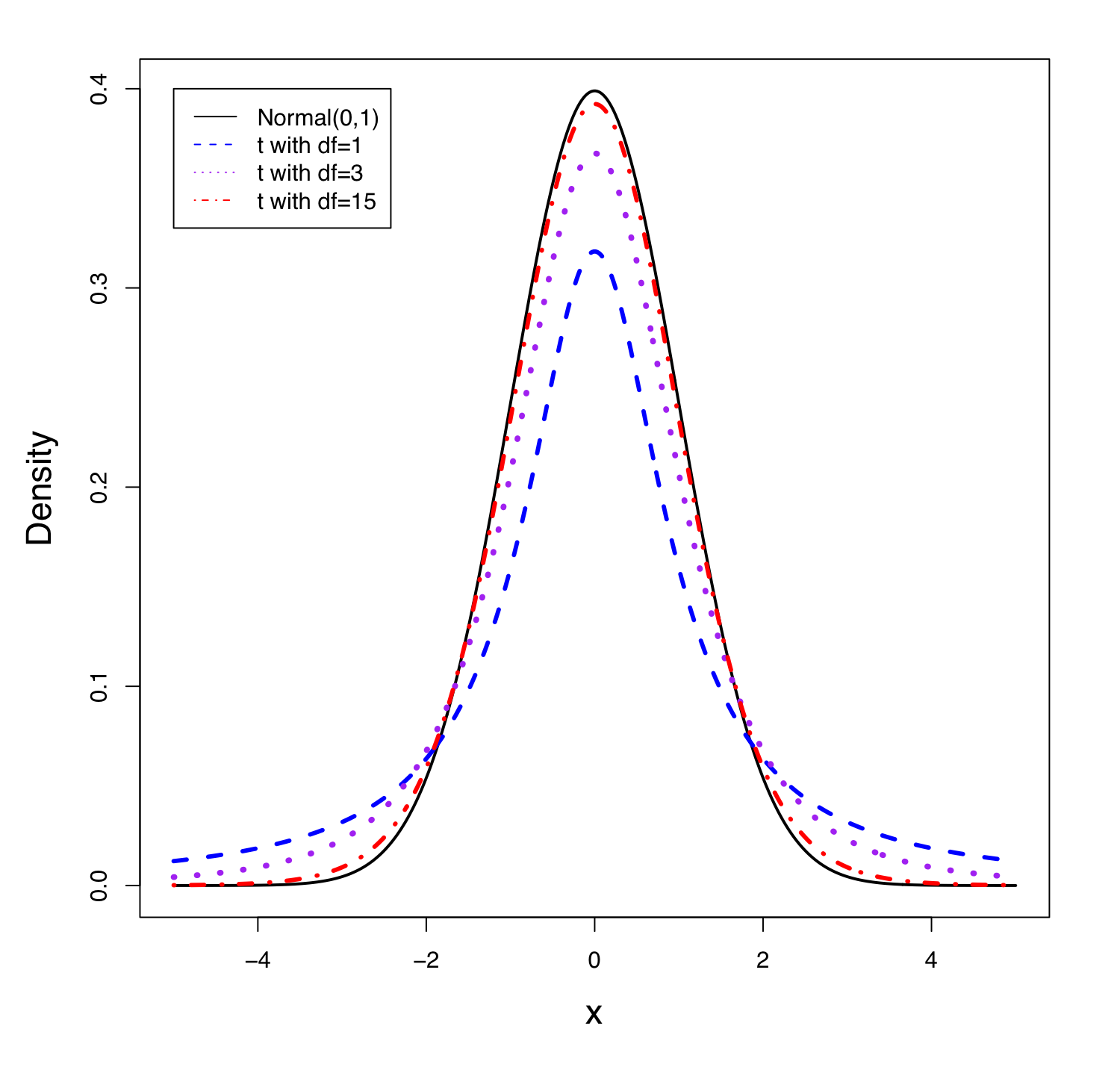
The t density curve is very similar to the standard normal density curve. The following figure shows several t density curves with different degrees of freedom and the standard normal density curve.
Here are the properties of a t distribution:
Key Facts: Properties of t Density Curve
- The total area under the curve is 1.
- Bell-shaped and symmetric at 0, that is, the area to the right of any given t-score is the same as the area to the left of its negative counterpart: [latex]P(t \: > \: t_{\alpha}) = P(t \: < \: -t_{\alpha})[/latex]. For example, [latex]P(t>2)=P(t<-2)[/latex].
- When the degrees of freedom [latex]df = n-1[/latex] increases, the t distribution approaches the standard normal distribution. When [latex]df = \infty[/latex], the t distribution becomes the standard normal.
- The standard normal curve is taller and slimmer, and the t distribution has a fatter and wider tail.
Unlike the standard normal table (Table II) whose main body gives left-tailed areas under the standard normal density curve, the main body of the t-score table (Table IV) gives t-scores, [latex]t_{\alpha}[/latex], which are defined in a manner analogous to [latex]z_{\alpha}[/latex]. That is, the t-scores [latex]t_{\alpha}[/latex] is the value such that the area to its right is [latex]\alpha[/latex], under the density curve of the t distribution with a given degree of freedom.
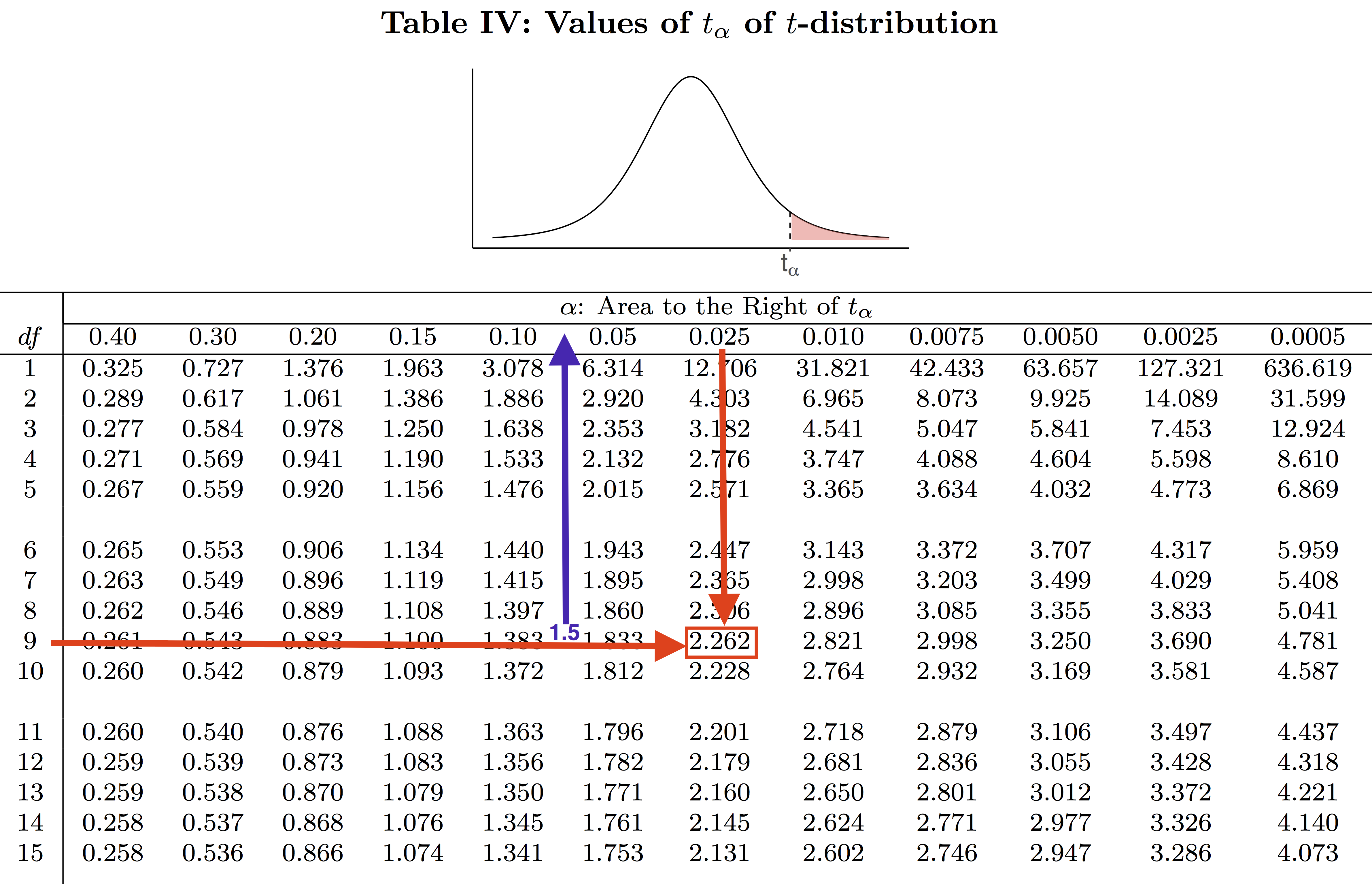
For example, if [latex]n=10[/latex] and [latex]df = n-1 = 9[/latex], then [latex]t_{0.025} = 2.262[/latex]. That is, the t-score 2.262 has an area of 0.025 to its right, under the t-density curve with 9 degrees of freedom. Notice that for each [latex]df[/latex], the t-table lists only 12 t-scores. For this reason, we are often required to approximate the area to the right of a given t-score. For example, to find the area to the right of the t-score 1.5 under the t density curve with [latex]df = 9[/latex], we first locate the t-score 1.5, which is between 1.383 and 1.833; then, if we look at the top of the table, we see that the area to the right of 1.5 is between 0.1 and 0.05. If we use technology, for example, the R commander, we determine that the t-score of 1.5 has a right-tailed area of 0.0839. That is, when [latex]df=9[/latex], [latex]t_{0.0839} = 1.5[/latex].

Exercise: Use of the t-Score Table
Given that [latex]n =15[/latex], use the t-score table (Table IV) to find
- [latex]t_{0.025}[/latex]
- [latex]t_{0.005}[/latex]
- [latex]P(t \geq 2.145)[/latex], which is the area to the right of 2.145 under the t density curve.
- [latex]P(t \leq -2.145)[/latex], which is the area to the left of -2.145 under the t density curve.
- [latex]P(t \geq 2.5)[/latex] , which is the area to the right of 2.5 under the t density curve.
Show/Hide Answer
For [latex]n=15, df= n-1 = 14[/latex]. Hence, we may refer to the bottom row of the table in Figure 7.4 and Figure 7.5.
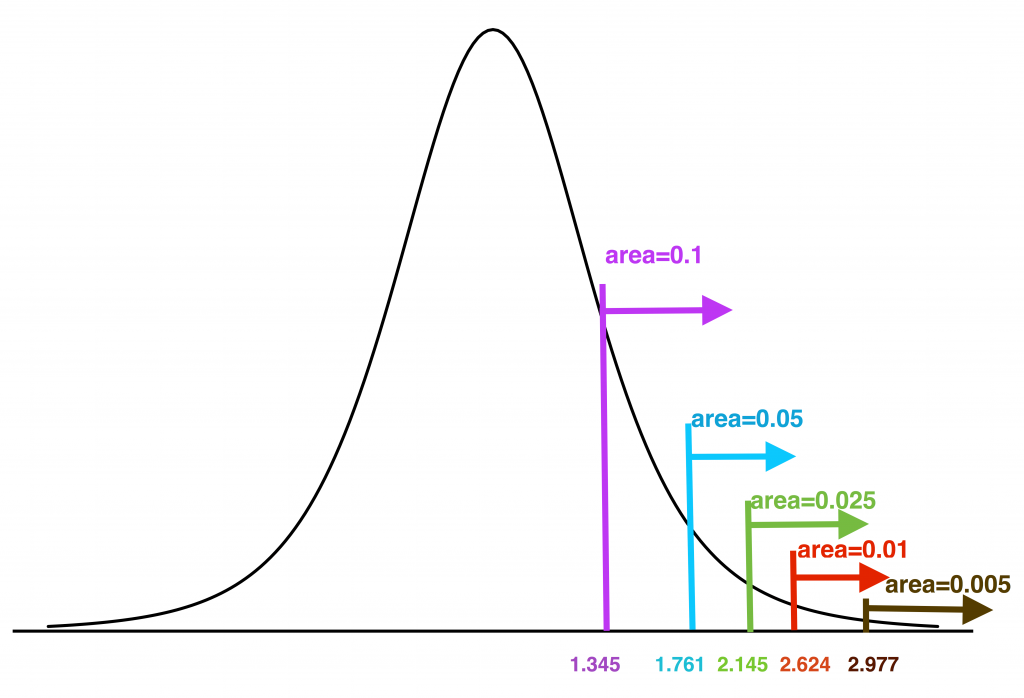
- [latex]t_{0.025} = 2.145[/latex]
- [latex]t_{0.005} = 2.977[/latex]
- Since [latex]t_{0.025}=2.145[/latex], it follows that [latex]P(t \geq 2.145) = 0.025[/latex].
- First note that the t distribution is symmetric at 0, so the area to the left of -2.145 is the same as the area to the right of 2.145. Therefore, [latex]P(t \leq -2.145) = P(t \geq 2.145) = 0.025[/latex], which is the area under the t density curve to the left of –2.145.
- Since 2.145 (which is [latex]t_{0.025}[/latex]) [latex]< 2.5 < 2.624[/latex] (which is [latex]t_{0.01}[/latex]), the area to the right of 2.5 should be somewhere between 0.025 and 0.01. That is, [latex]0.01 < P(t \geq 2.5) < 0.025[/latex].
7.2.2 One-Sample t Interval When σ is Unknown
When the population standard deviation [latex]\sigma[/latex] is unknown and estimated by the sample standard deviation [latex]s[/latex], a [latex](1-\alpha) \times 100\%[/latex] confidence interval is given by a one-sample t interval:
Assumptions:
- A simple random sample (SRS)
- Normal population or large sample size (rule of thumb: [latex]n \ge 30[/latex])
- The population standard deviation [latex]\sigma[/latex] is unknown
Formula: [latex](\bar{x} - t_{\alpha / 2} \frac{s}{\sqrt{n}}, \bar{x} + t_{\alpha / 2}\frac{s}{\sqrt{n}})[/latex] or [latex]\bar x \pm t_{\alpha/2}\frac{s}{\sqrt{n}}[/latex]
Interpretation: We are [latex](1-\alpha) \times 100\%[/latex] confident that the interval contains the population mean [latex]\mu[/latex].
Example: One-Sample t Interval
A computer company claims that the average lifetime of its laptops is about 4 years. A simple random sample of 36 laptops yields an average lifetime of 3.5 years with a sample standard deviation of 4.2 years.
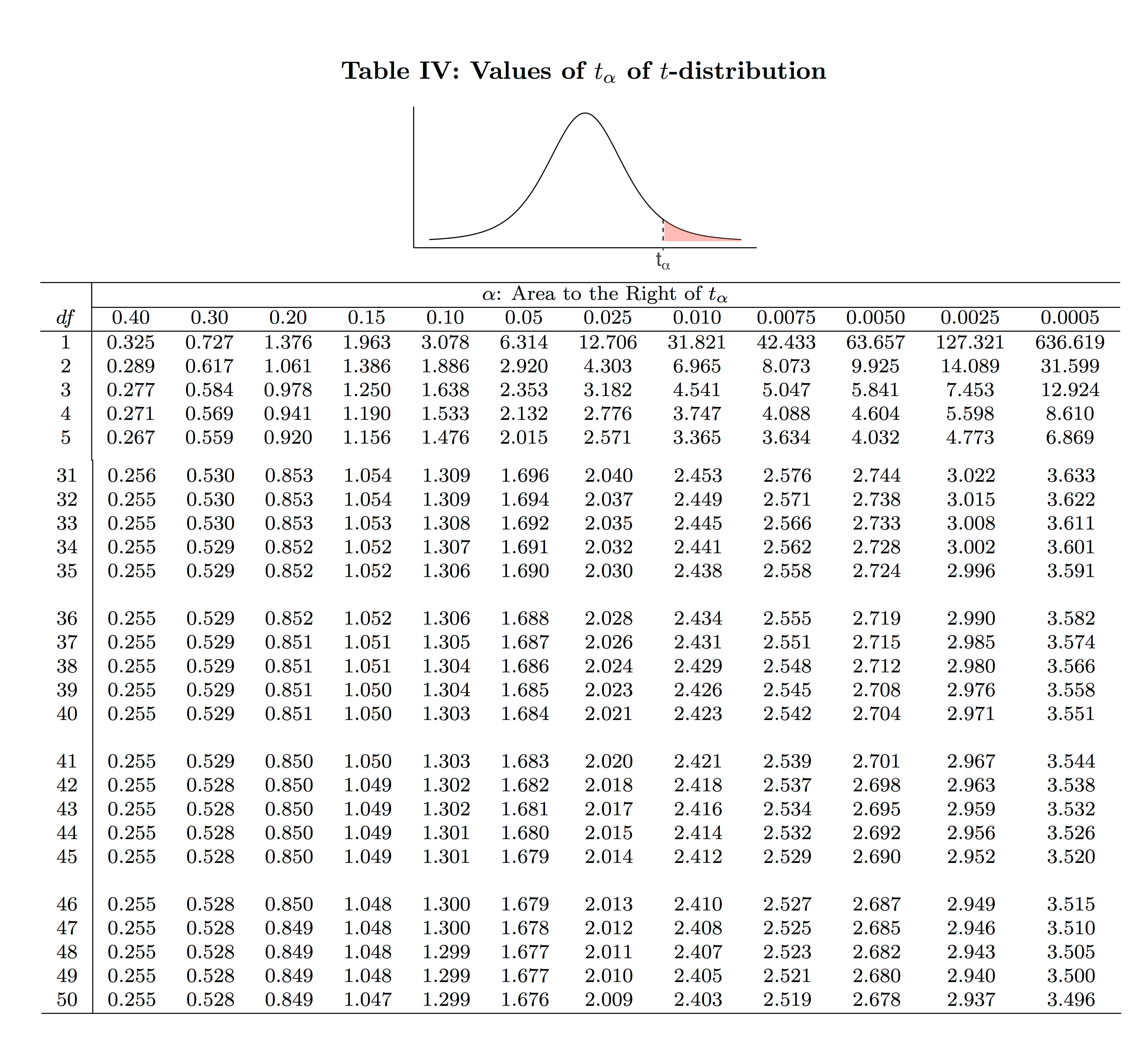
You could use the following truncated Table IV to obtain the t-scores.
- Obtain a 99% confidence interval for the population mean lifetime [latex]\mu[/latex].
Check the assumptions:- We have a simple random sample (SRS).
- We do not know whether the population is normal or not, but we have a large sample size [latex]n = 36 > 30[/latex].
- [latex]\sigma[/latex] is unknown and estimated by [latex]s=4.2[/latex].
Steps:
- Find [latex]t_{\alpha / 2}[/latex]: [latex]n = 36, df = n-1 = 36-1 = 35[/latex] [latex]1 - \alpha = 0.99 \Longrightarrow \alpha = 0.01 \Longrightarrow \frac{\alpha}{2} = 0.005 \Longrightarrow t_{\alpha / 2} = t_{0.005} = 2.724[/latex] (using Table IV).
- Information: [latex]n = 36, \bar{x} = 3.5, s = 4.2[/latex].
- Interval: [latex]\begin{align*}\bar{x} \pm t_{\alpha / 2} \frac{s}{\sqrt{n}}&= 3.5 \pm 2.724 \times \frac{4.2}{\sqrt{36}}=(3.5-1.9068, 3.5+1.9068 )\\&=(1.5932, 5.4068).\end{align*}[/latex]
Interpretation: We are 99% confident that the interval [latex](1.5932, 5.4068)[/latex] contains the population mean lifetime. In other words, we are 99% confident that this computer company produces laptops with a mean lifetime somewhere between 1.5932 and 5.4068 years.
- Obtain an 80% confidence interval for the population mean lifetime.
Steps:- Find [latex]t_{\alpha / 2}[/latex] : [latex]n = 36, df = n-1 = 36-1 = 35[/latex] [latex]1 - \alpha = 0.8 \Longrightarrow \alpha = 0.2. \Longrightarrow \frac{\alpha}{2} = 0.1 \Longrightarrow t_{\alpha / 2} = t_{0.1} = 1.306[/latex] (using Table IV).
- Information: [latex]n = 36, \bar{x} = 3.5, s = 4.2[/latex].
- Interval:
[latex]\begin{align*}\bar{x} \pm t_{\alpha / 2} \frac{s}{\sqrt{n}}&= 3.5 \pm 1.306 \times \frac{4.2}{\sqrt{36}}= ( 3.5 - 0.9142, 3.5 + 0.9142)\\ &= (2.5858, 4.4142 ).\end{align*}[/latex]
Interpretation: We are 80% confident that the interval [latex](2.5858, 4.4142)[/latex] contains the population mean life [latex]\mu[/latex]. In other words, we are 80% confident that this computer company produces laptops with a mean lifetime somewhere between 2.5858 and 4.4142 years.
- Does the confidence interval in part a) provide any evidence against the company’s claim that the average lifetime of this brand of laptops is about 4 years?
No. Since the interval [latex](1.5932, 5.4068)[/latex] contains 4, we can not reject the claim that the average lifetime is about 4 years.
Exercise: One-Sample t Interval
A nutrition laboratory tests 50 “reduced sodium” hot dogs and finds the sample mean sodium content is 300 mg, with a sample standard deviation of 36 mg.
- Obtain a 90% confidence interval for the mean sodium content of this brand of hot dog.
- Interpret the confidence interval obtained in part (a).
- Suppose that the mean sodium content of all brands of hot dogs on the market is 320 mg. Can we claim that this brand of “reduced sodium” hot dogs has a lower average sodium content?
Show/Hide Answer
Answers:
- Steps:
- Find [latex]t_{\alpha / 2}[/latex] : [latex]n = 50, df = n-1 = 50 -1 = 49[/latex] [latex]1 - \alpha = 0.9 \Longrightarrow \alpha = 0.1 \Longrightarrow \frac{\alpha}{2} = 0.05 \Longrightarrow t_{\alpha / 2} = t_{0.05} = 1.677[/latex] (using Table IV).
- Information: [latex]n = 50, \bar x = 300, s= 36[/latex].
- Interval:
[latex]\begin{align*}\bar{x} \pm t_{\alpha / 2} \frac{s}{\sqrt{n}} &= 300 \pm 1.677 \times \frac{36}{\sqrt{50}} = (300 - 8.538, 300 + 8.538)\\& = (291.462, 308.538 ).\end{align*}[/latex]
- Interpretation: We are 90% confident that this brand of “reduced sodium” hot dogs has a mean sodium content somewhere between 291.462 mg and 308.538 mg.
- Since the entire interval [latex](291.462, 308.538)[/latex] is below 320 mg, we have evidence that this brand of “reduced sodium” hot dog has a lower average sodium content than 320 mg.
