13.6 The Coefficient of Determination
Continuing the used car example, observe that the prices of the 15 cars are different, so we can quantity the variation among prices [latex]y_i[/latex] by looking at the distance between each observation and the mean, i.e., [latex](y_i - \bar{y})^2[/latex]. Therefore, the total variation of prices is calculated by [latex]SST = \sum_{i=1}^n (y_i - \bar{y})^2[/latex]. The term SST is called the total sum of squares. The prices of the 15 used cars are different; part of the reason is that their ages are different, so that means “age” explains some of the variation in “price”.
It can be shown that the total variation in the response [latex]y[/latex] (SST, which is the total sum of squares) can be decomposed into two parts: variation explained by predictor variable [latex]x[/latex] through the regression equation (SSR, which is the regression sum of squares) and the variation not explained by [latex]x[/latex] (SSE, which is the error sum of squares), i.e.,
[latex]\begin{aligned} SST & = \sum (y_i - \bar{y})^2 \\ & = \sum (y_i - \hat{y}_i + \hat{y}_i - \bar{y})^2 \\ & = \sum (y_i - \hat{y}_i)^2 + \sum (\hat{y}_i - \bar{y})^2 \\ & = SSE + SSR. \end{aligned}[/latex]
The sums of squares are similar to ANOVA, and have a similar decomposition. The distance from [latex]y_i[/latex] to [latex]\bar{y}[/latex] is composed of two parts: the distance from [latex]y_i[/latex] to [latex]\hat{y}_i[/latex] and the distance from [latex]\hat{y}_i[/latex] to [latex]\bar{y}[/latex]. The difference between [latex]y_i[/latex] and [latex]\hat{y}_i[/latex] is the residual [latex]e_i = y_i - \hat{y}_i[/latex]. Then we have [latex]SST = SSE + SSR[/latex] with
[latex]SST = \sum (y_i - \bar{y})^2 = S_{yy}, SSE = \sum (y_i - \hat{y}_i)^2 = \sum e_i^2, SSR = \sum (\hat{y}_i - \bar{y})^2 = r^2 S_{yy} = \frac{S_{xy}^2}{S_{xx}}[/latex].
The square of the correlation coefficient, [latex]R^2 = r^2[/latex], is called the coefficient of determination. It can be shown that
[latex]r^2 = \frac{S_{xy}^2}{S_{xx} \times S_{yy}} = \frac{SSR}{SST}[/latex].
The coefficient of determination [latex]r^2[/latex] indicates the percentage of total variation (SST) in the observed response variable that is explained by the predictor variable [latex]x[/latex] through the regression equation (SSR).
Example: Correlation Coefficient and Coefficient of Determination
Given the summaries of the 15 used cars,
[latex]n = 15, \sum x_i = 92, \sum x_i^2 = 724, \sum y_i = 125, \sum y_i^2 = 1193, \sum x_i y_i = 616.[/latex]
- Calculate and interpret the correlation coefficient [latex]r[/latex].
[latex]\begin{align*}S_{xy} &= \sum x_i y_i - \frac{\left( \sum x_i \right) \left( \sum y_i \right) }{n} = 616 - \frac{92 \times 125}{15} = -150.667,\\S_{xx} &= \sum x_i^2 - \frac{ \left( \sum x_i\right)^2 }{n} = 724 - \frac{92^2}{15} = 159.733,\\S_{yy} &= \sum y_i^2 - \frac{ \left( \sum y_i \right)^2 }{n} = 1193 - \frac{125^2}{15} = 151.333,\\r& = \frac{S_{xy}}{\sqrt{S_{xx} \times S_{yy}}} = \frac{-150.667}{159.733 \times 151.333} = -0.9691.\end{align*}[/latex]
Interpretation: There is a strong, negative, linear association between the price and the age of the used cars.
- Calculate and interpret the coefficient of determination [latex]r^2[/latex].
[latex]r^2 = (-0.9691)^2 = 0.9391[/latex].
Interpretation: 93.91% of the variation in the observed price of the used cars is due to the age of the used cars. That is, 93.91% of the variation in the price of the used cars can be explained by the age of the used cars through the regression equation.
Note: A common mistake in interpreting [latex]r^2[/latex] is that 93.91% of the points lie on a straight line.
Note: the geometric interpretation of [latex]r^2[/latex] is NOT required for STAT 151; the remaining material of this section is only for students interested in explaining the decomposition.
The following figure shows the geometric interpretation of the decomposition [latex]SST=SSR+SSE[/latex], i.e.,
[latex]||\mathbf{Y-\bar Y}||^2=||\mathbf{\hat Y-\bar Y}||^2+||\mathbf{Y-\hat Y}||^2[/latex]
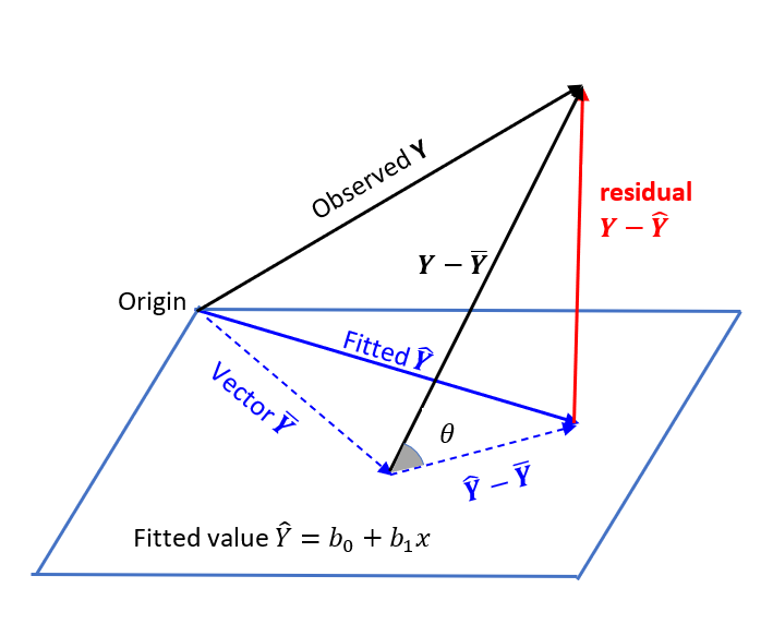
Suppose there are [latex]n[/latex] observations [latex]\{x_i, Y_i\}_{i=1}^n[/latex] in a regression problem. The responses [latex](Y_1, Y_2, \cdots, Y_n)^T[/latex] forms an [latex]n\times 1[/latex] vector [latex]\mathbf{Y}[/latex]. The fitted values [latex](\hat Y_1, \hat Y_2, \cdots, \hat Y_n)^T[/latex] is an orthogonal projection of the observed [latex]\mathbf{Y}[/latex] onto the plane of the predictor variable [latex]\mathbf{x}=(x_1, x_2, \cdots, x_n)^T[/latex]. Since the residual vector [latex]\mathbf{Y}-\mathbf{\hat Y}[/latex] is orthogonal to the plane, the triangle formed with edges [latex]\mathbf{Y}-\mathbf{\bar Y}[/latex], [latex]\mathbf{\hat Y}-\mathbf{\bar Y},[/latex] and [latex]\mathbf{Y}-\mathbf{\hat Y}[/latex] is a right triangle. Therefore,
[latex]||\mathbf{Y-\bar Y}||^2=||\mathbf{\hat Y-\bar Y}||^2+||\mathbf{Y-\hat Y}||^2.[/latex]
Let [latex]\theta[/latex] be the angle between the two vectors [latex]\mathbf{Y}-\mathbf{\bar Y}[/latex] and [latex]\mathbf{\hat Y}-\mathbf{\bar Y}[/latex]. It can be shown that
[latex]r^2=\cos^2 \theta=\frac{||\mathbf{\hat Y}-\mathbf{\bar Y}||^2}{||\mathbf{Y}-\mathbf{\bar Y}||^2}=\frac{SSR}{SST}.[/latex]
