Suppose the variable of interest is X and the population consists of N individuals. The possible values of X are the different measurements for each individual in the population. For example, suppose the variable of interest is X=height and the population is the N = 60 students in our class. The number N = 60 is called the population size. Suppose we measure each student’s height and draw a histogram of those N = 60 measurements. In that case, the resulting distribution is the population distribution, that is, the distribution of the random variable X. The average height of all 60 students is the population mean [latex]\mu[/latex].

We often use the sample mean [latex]\bar{X}[/latex] to estimate the population mean [latex]\mu[/latex]. However, since the observed value of [latex]\bar{X}[/latex] varies from sample to sample, it is helpful to know the typical accuracy of this estimator. For example, how confident are we that the error in estimating [latex]\mu[/latex] by [latex]\bar{x}[/latex] is at most 2 cm? To answer this kind of question, we need to know the distribution of the sample mean [latex]\bar{X}[/latex].

For a population of size N, if we take a sample of size n, there are [latex]\binom{N}{n}[/latex] distinct samples, each of which gives one possible value of the sample mean [latex]\bar x[/latex]. The [latex]\binom{N}{n}[/latex] values of [latex]\bar{x}[/latex] give the distribution of the sample mean [latex]\bar{X}[/latex], which is also called the sampling distribution of the sample mean. A histogram of the [latex]\binom{N}{n}[/latex] values of [latex]\bar{x}[/latex] shows the distribution of [latex]\bar{X}[/latex].  However, [latex]\binom{N}{n}[/latex] is often so large that we are unable to consider all possible samples of size n directly. Fortunately, we can still obtain a reasonable approximation of the distribution of [latex]\bar{X}[/latex] by obtaining a large number of random samples, say 10,000, computing each sample mean, and drawing a histogram based on our sample of the sample means. For example, if the population size is N = 60 and the sample size is n = 5, there are [latex]\binom{N}{n} = _{60}C_5 = 5,461,512[/latex] different samples, many of which have different values of [latex]\bar{x}[/latex]. Drawing a histogram of these 5,461,512 [latex]\bar{x}[/latex] values gives the distribution of the sample mean [latex]\bar{X}[/latex], with sample size n = 5. Moreover, the sampling distribution of the sample mean [latex]\bar{X}[/latex] can be described in three aspects: centre, spread (variation), and shape.

6.2.1 Mean and Standard Deviation of the Sample Mean

Let’s consider a population consisting of 5 students. Suppose their heights (in cm) are [latex]x_1 = 155, x_2= 165, x_3=175, x_4=185, x_5=195[/latex]. The population size is N=5 and the population mean [latex]\mu[/latex] and population standard deviation [latex]\sigma[/latex] are: [latex]\begin{align*} \mu &= \frac{\sum x_i}{N} \\  &= \frac{155+165 + 175 + 185 +195}{5} \\ &= 175, \\ \sigma &= \sqrt{ \frac{ \sum (x_i - \mu )^2 }{N} } \\ &= \sqrt{\frac{(155-175)^2 + (165 -175)^2 + (175 - 175)^2 + (185 - 175)^2 + (195-175,)^2} {5} } \\ &= 14.14. \end{align*}[/latex]

Consider a simple random sample of size n = 2, which means randomly picking two students from this population of five students. n = 2  is called the sample size. The number of ways we can pick two students out of five is [latex]_5C_2 = \binom{5}{2} = 10[/latex]. For example, one possible sample is [latex]\{x_1, x_2\}[/latex] which gives a value of the sample mean,

[latex]\bar{x} = \frac{x_1 + x_2}{2} = \frac{155+ 165}{2} =  160[/latex].

Another possible sample is [latex]\{x_1, x_3 \}[/latex]  and the corresponding value of the sample mean is:

[latex]\bar{x} = \frac{x_1 + x_3}{2} = \frac{155+ 175}{2} = 165.[/latex]

Table 6.1 lists all possible samples of sample size n = 2, 3, 4 and their corresponding sample mean values. The mean and standard deviation of the sample mean of all possible sample sizes are also given in the table.

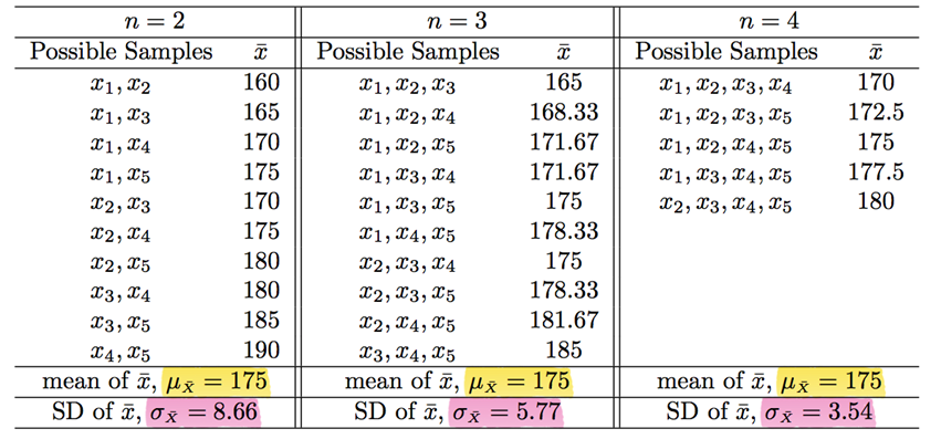
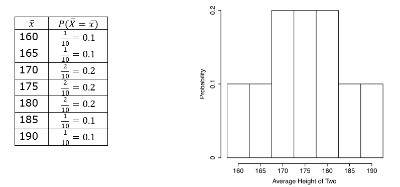
The mean and standard deviation of the sample mean [latex]\bar{X}[/latex] are denoted as [latex]\mu_{\bar{X}}[/latex] and [latex]\sigma_{\bar{X}}[/latex] respectively. When the sample size [latex]n=2[/latex], Table 6.1 shows 10 possible values of the sample mean: [latex]160, 165, \cdots, 185, 190[/latex]; there is one value of 160 and two values of 180, giving the probabilities of [latex]\frac{1}{10}[/latex] and [latex]\frac{2}{10}[/latex] observing these two values respectively. The probability distribution and distribution histogram of the sample mean [latex]\bar{X}[/latex] with [latex]n=2[/latex] are:

The mean and the standard deviation of the sample mean with n = 2 are:

[latex]\begin{align*} \mu_{\bar{X}} &= \frac{160 + 165 + 170 + 175+ 170 + 175 + 180 + 180 + 185 + 190}{10} \\ &= 175, \\ \sigma_{\bar{X}} &= \sqrt{ \frac{\sum (\bar{x} - \mu_{\bar{X}})^2}{N}} \\ &= \sqrt{ \frac{ (160-175)^2 + (165-175)^2 + ... + (185 - 175)^2 + (190 - 175)^2}{10} } \\ &= 8.66. \end{align*}[/latex]

When the sample size is n = 3, the mean and the standard deviation of the sample mean are:

[latex]\begin{align*} \mu_{\bar{X}} &= \frac{165 + 168.33 + 171.67 + 171.67+ 175 + 178.33 + 175 + 178.33 + 181.67 + 185}{10} \\ &= 175, \\ \sigma_{\bar{X}} &= \sqrt{ \frac{\sum (\bar{x} - \mu_{\bar{X}})^2}{N}} \\ &= \sqrt{ \frac{ (160-175)^2 + (168.33-175)^2 + ... + (185 - 175)^2 + (190 - 175)^2}{10} } \\ &= 5.77. \end{align*}[/latex]

When the sample size is n = 4, the mean and the standard deviation of the sample mean are:

[latex]\begin{align*} \mu_{\bar{X}} &= \frac{170 +172.5 +175 +177.5 + 180 }{5} \\ &= 175, \\ \sigma_{\bar{X}} &= \sqrt{ \frac{\sum (\bar{x} - \mu_{\bar{X}})^2}{N}} \\ &= \sqrt{ \frac{ (170-175)^2 + (172.5-175)^2 + (175 - 175)^2 + (177.5 - 175)^2 + (180 - 175)^2}{5} } \\ &= 3.54. \end{align*}[/latex]

The above results show that the mean of the sample mean equals the population mean regardless of the sample size, i.e., [latex]\mu_{\bar{X}} = \mu[/latex], while the standard deviation of the sample mean decreases when the sample size n increases. It can be shown that when sampling without replacement from a finite population, like those listed in Table 6.1,

[latex]\sigma_{\bar{X}} = \sqrt{ \frac{N-n}{N-1} } \times \frac{\sigma}{\sqrt{n}}.[/latex]

If we instead sample with replacement from a finite population, the standard deviation of the sample mean is

[latex]\sigma_{\bar{X}} = \frac{\sigma}{\sqrt{n}}.[/latex]

Note: If we sample without replacement, [latex]\sigma_{\bar{X}}[/latex] is approximately equal to [latex]\frac{\sigma}{\sqrt{n}}[/latex], as long as the sample size n is much smaller than the population size N. For simplicity of notation, we only focus on the sample without replacement case for the distribution of the sample mean in the remaining chapters.

6.2.2 Shape of the Distribution of the Sample Mean (Central Limit Theorem)

We discuss the shape of the distribution of the sample mean for two cases: when the population distribution is normal, i.e., the variable of interest [latex]X \sim N(\mu, \sigma)[/latex] and when the population distribution is not normal.

When the Population is Normally Distributed

Suppose the random variables [latex]X_1, X_2, \dots, X_n[/latex] represent a simple random sample from a normal population distribution [latex]N(\mu, \sigma)[/latex], then the sample mean

[latex]\bar{X} = \frac{X_1 + X_2 + \dots + X_n}{n}[/latex]

also follows a normal distribution, regardless of the value of the sample size [latex]n[/latex]. This is a consequence of the fact that a linear combination of normal random variables is itself a normal random variable.

Example: Grade of 100 Students

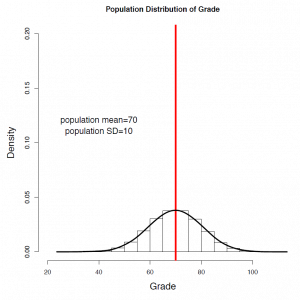
Suppose a population consists of 100 students and the variable of interest is [latex]X=[/latex] student grades. Due to bonus questions, the maximum grade might be above 100. The histogram of the grades of these 100 students gives the population (or parent) distribution, or simply the distribution of [latex]X[/latex]. The mean and standard deviation of these 100 grades give the population mean and population standard deviation [latex]\mu = 70, \sigma = 10[/latex]. It is reasonable for us to assume grades follow a normal distribution since the histogram is bell-shaped and the points in the QQ plot form an approximate straight-line pattern.

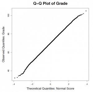Figure 6.2: Density and Normal Probability Plot of Grade (Population). [Image Description (See Appendix D Figure 6.2)]

 

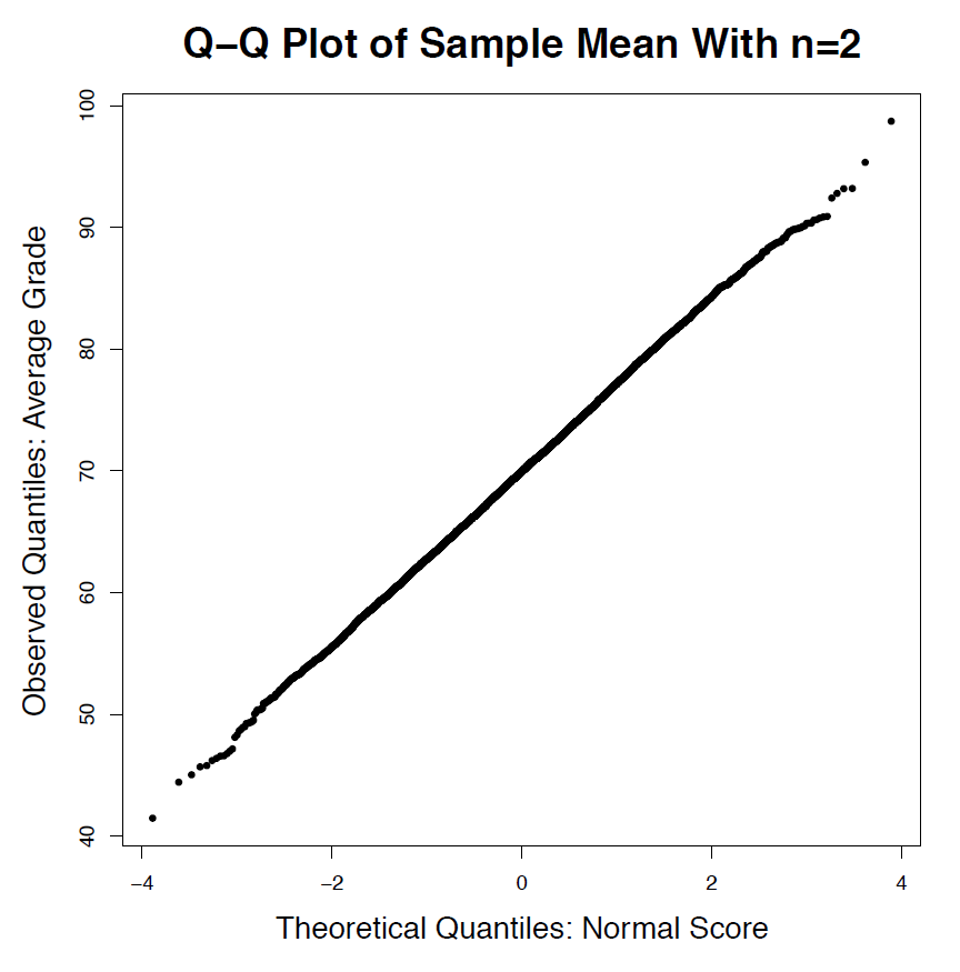
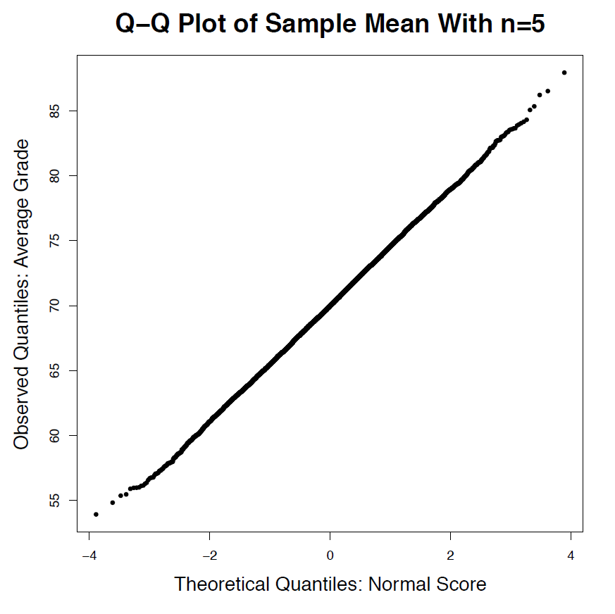
Let’s examine the distributions of the sample mean [latex]\bar{X}[/latex] for sample size [latex]n = 2, 5, 30[/latex]. In each histogram, the red solid line indicates the population mean and the blue dashed line indicates the mean of the sample mean. Recall the steps to obtain the distribution of the sample mean:

1. Obtain a sample of size n from the population of 100 students and calculate the sample mean [latex]\bar x =[/latex] average grade for this particular sample.
2. Repeat step 1 for each of the [latex]\binom{100}{n}=_{100}C_n[/latex] different samples to obtain [latex]\binom{100}{n}[/latex] sample means [latex]\bar x[/latex] values.
3. Draw a histogram of those [latex]\binom{100}{n}[/latex] sample means.
4. If [latex]\binom{100}{n}[/latex] is too large, then we can approximate the distribution of the sample mean by performing the above steps using a large number of random samples (say 10,000), instead of all [latex]\binom{100}{n}[/latex] samples.

Note that the mean and standard deviation are [latex]\mu_{\bar{X}} = \mu = 70, \sigma_{\bar{X}} = \frac{\sigma}{\sqrt{n}} = \frac{10}{\sqrt{n}}.[/latex]

[latex]\sigma_{\bar{X}} = \frac{\sigma}{\sqrt{n}} = \frac{10}{\sqrt{2}} = 7.07[/latex]	[latex]\sigma_{\bar{X}} = \frac{\sigma}{\sqrt{n}} = \frac{10}{\sqrt{5}} =4.47[/latex]	[latex]\sigma_{\bar{X}} = \frac{\sigma}{\sqrt{n}} = \frac{10}{\sqrt{30}} = 1.83[/latex]

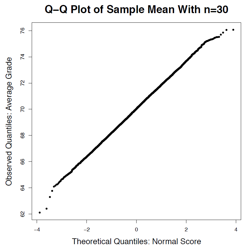Figure 6.3: Density and Normal Probability Plot of the Average Grade (Sample Mean) for n=2, 5, 30. [Image Description (See Appendix D Figure 6.3)] Click on the image to enlarge it.

For each sample size, we can verify the following:

• The distribution of the sample mean [latex]\bar{X}[/latex] is approximately normally distributed (symmetric, bell shape, unimodal);
• The mean of the sample mean equals the population mean of 70, and the standard deviation of the sample mean gets smaller and smaller when sample size n increases and roughly equals the population standard deviation divided by the square root of the sample size. Note that they are approximately equal because we have obtained 10,000 random samples for each sample size n, instead of all [latex]\binom{100}{n}=_{100}C_n[/latex] possible samples.

When the Population is not Normally Distributed

To illustrate two non-normal populations, we will discuss the uniform distribution (which is symmetric) and the exponential distribution (which is extremely right-skewed).

Example: Population Distribution is Uniform (Symmetric but not Normal)

Consider rolling a fair die. Since the die is fair, each face has the same chance to be observed; therefore, the population distribution is a uniform distribution with the following probability distribution.

Table 6.2: Working Table for the Population Mean and Standard Deviation [latex]\small{x}[/latex] [latex]\small{P(X=x)}[/latex] [latex]\small{xP(X=x})[/latex] [latex]\small{x^2P(X=x)}[/latex] [latex]\small{1}[/latex] [latex]\small{1/6}[/latex] [latex]\small{1/6}[/latex] [latex]\small{1^2\times \frac{1}{6} = 1/6}[/latex] [latex]\small{2}[/latex] [latex]\small{1/6}[/latex] [latex]\small{2/6}[/latex] [latex]\small{2^2\times \frac{1}{6} = 4/6}[/latex] [latex]\small{3}[/latex] [latex]\small{1/6}[/latex] [latex]\small{3/6}[/latex] [latex]\small{3^2\times \frac{1}{6} = 9/6}[/latex] [latex]\small{4}[/latex] [latex]\small{1/6}[/latex] [latex]\small{4/6}[/latex] [latex]\small{4^2\times \frac{1}{6} = 16/6}[/latex] [latex]\small{5}[/latex] [latex]\small{1/6}[/latex] [latex]\small{5/6}[/latex] [latex]\small{5^2\times \frac{1}{6} = 25/6}[/latex] [latex]\small{6}[/latex] [latex]\small{1/6}[/latex] [latex]\small{6/6}[/latex] [latex]\small{6^2\times \frac{1}{6} = 36/6}[/latex] sum=1 sum=21/6=3.5 sum=91/6

The population mean and standard deviation are calculated as follows:

[latex]\begin{align*}  \mu &= \sum xP(X=x) \\ &= \frac{1}{6}(1 + 2+3+4+5+6) \\ &= 3.5, \\ \sigma &= \sqrt{\sum x^2 P(X=x) - \mu^2} \\ &= \sqrt{\frac{1}{6}(1^2 + 2^2 + 3^2 + 4^2 + 5^2 + 6^2 ) - 3.5^2} \\ &= 1.71. \end{align*}[/latex]

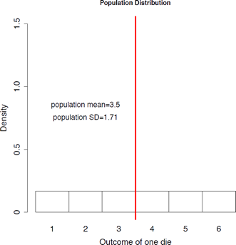
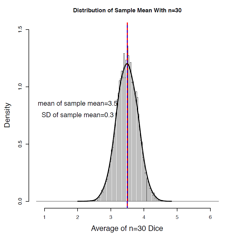
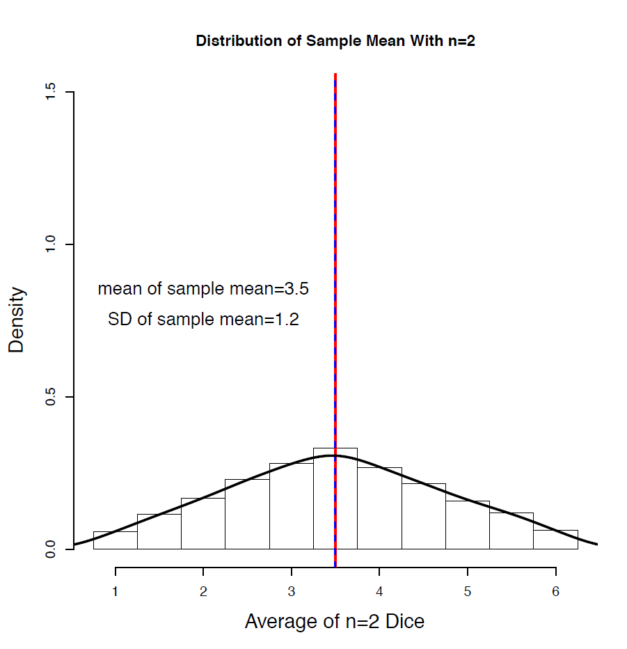
The uniform distribution is not bell-shaped and, hence, is not a normal distribution. Let’s examine the distribution of the sample mean with sample sizes n = 2, 5, 30, that is, the distribution of the average of n rolls of a fair die. Note that the mean and standard deviation are: [latex]\mu_{\bar{X}} = \mu = 3.5; \sigma_{\bar{X}} = \frac{\sigma}{\sqrt{n}} = \frac{1.71}{\sqrt{n}}[/latex].

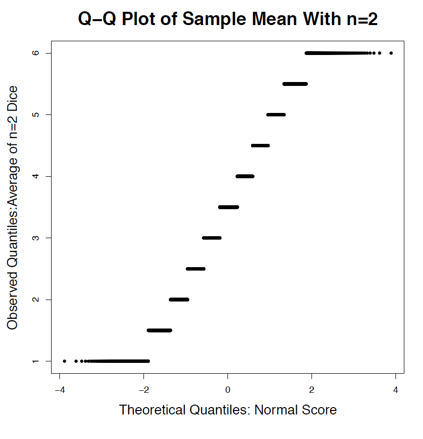
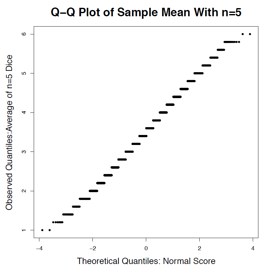
[latex]\sigma_{\bar{X}} = \frac{\sigma}{\sqrt{n}} = \frac{1.71}{\sqrt{2}} = 1.21[/latex] shape: triangular	[latex]\sigma_{\bar{X}} = \frac{\sigma}{\sqrt{n}} = \frac{1.71}{\sqrt{5}} = 0.76[/latex] shape: normal	[latex]\sigma_{\bar{X}} = \frac{\sigma}{\sqrt{n}} = \frac{1.71}{\sqrt{30}} = 0.31[/latex] shape: normal
Figure 6.5: Density and Normal Probability Plot of the Average of n=2, 5, 30 Rolls (Sample Mean). [Image Description (See Appendix D Figure 6.5)] Click on the image to enlarge it.

 

Here are the findings regarding the distribution of the sample mean [latex]\bar{X}[/latex]:

• The mean of the sample mean is 3.5, which equals the population mean regardless of the sample size n; the standard deviation roughly equals the population standard deviation divided by the square root of the sample size.
• Notice that for [latex]n=2[/latex], the distribution of the sample mean appears triangular (not normal), but it becomes increasingly normal for [latex]n=5[/latex] and [latex]n=30[/latex].

Example: Population Distribution is Exponential (Extremely Right Skewed)

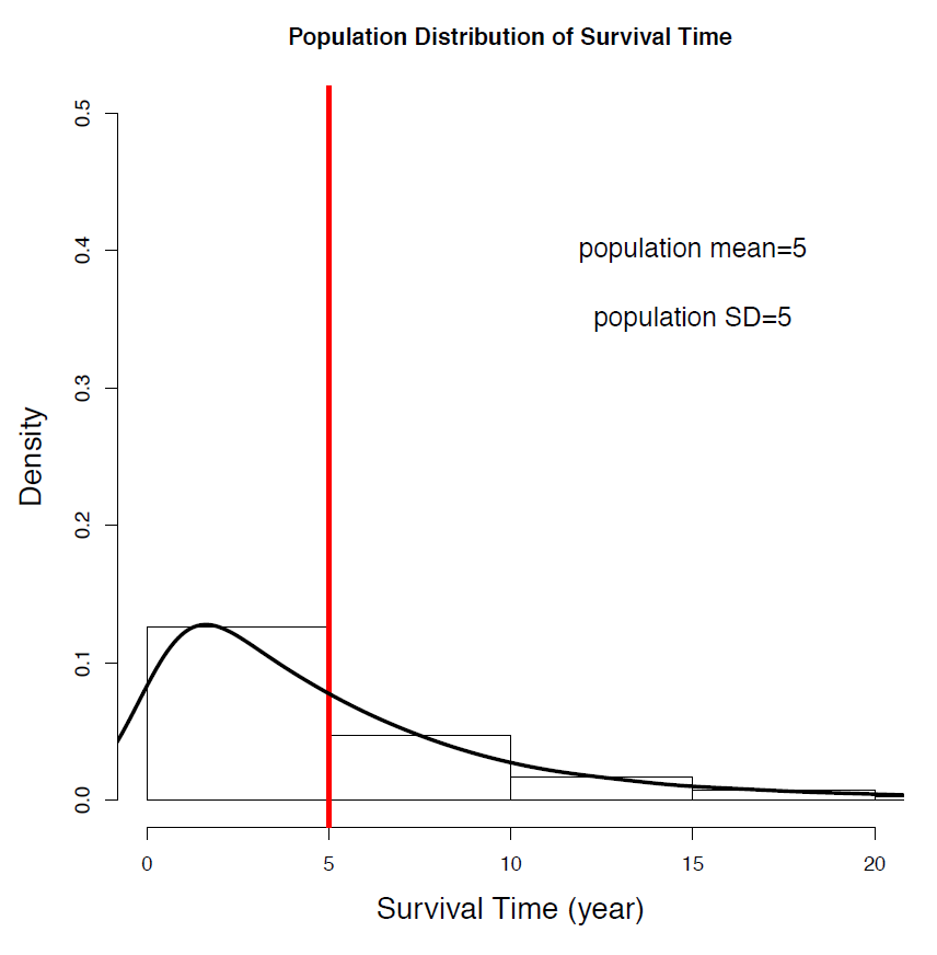
The exponential distribution is an extremely right-skewed distribution that appears in a variety of real-world applications, including survival times. Suppose [latex]X=[/latex]survival time of liver cancer patients, and that [latex]X[/latex] follows an exponential distribution with a mean and standard deviation of 5 years.

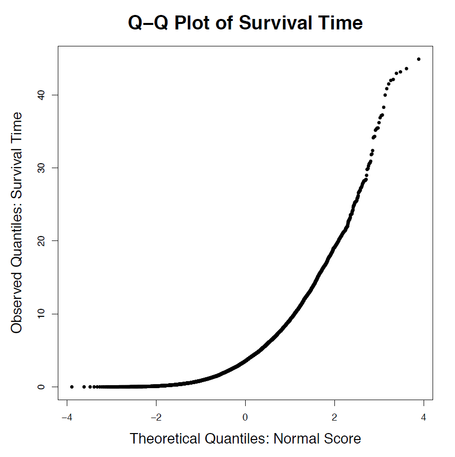Figure 6.6: Density and Normal Probability Plot of Survival Time (Population). [Image Description (See Appendix D Figure 6.6)]

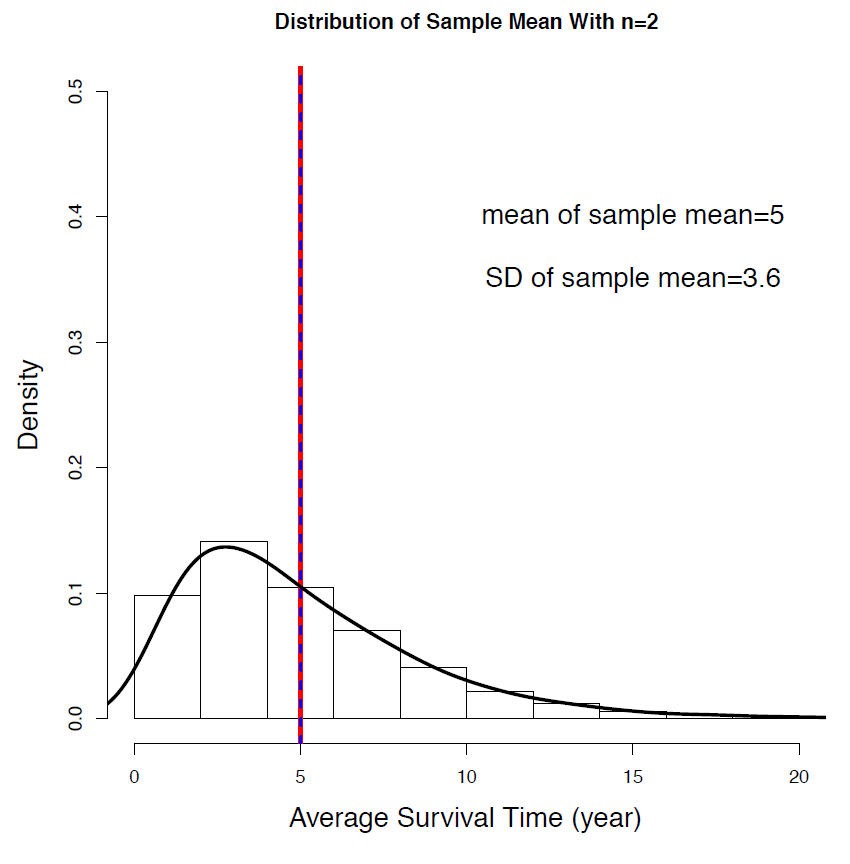
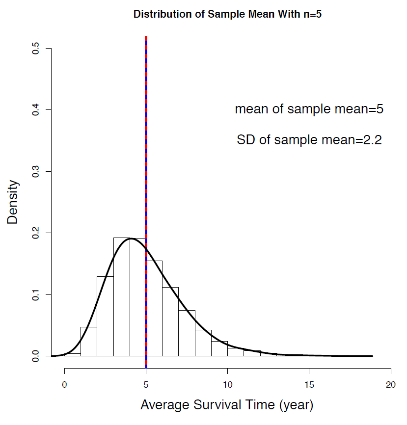
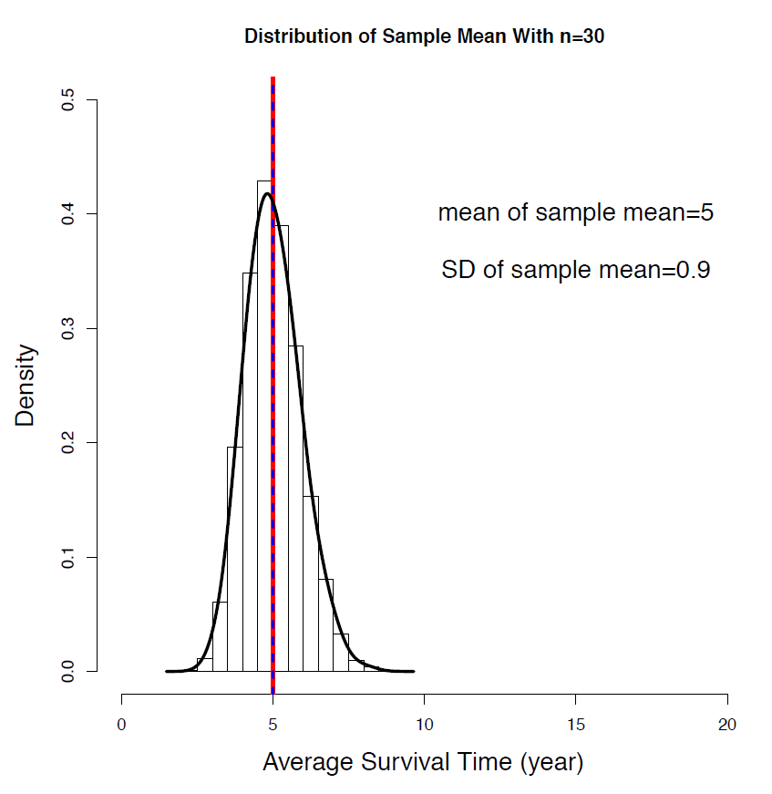
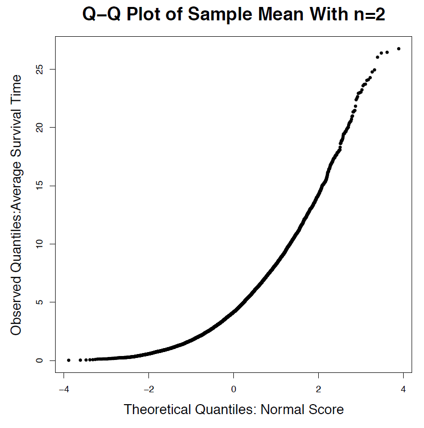
Let’s examine the distribution of the sample mean with sample sizes [latex]n= 2, 5, 30[/latex]. That is, the distribution of the average survival time of n randomly selected patients. Once again, note that the mean and standard deviation of the sample mean are: [latex]\mu_{\bar{X}} = \mu = 5; \sigma_{\bar{X}} = \frac{\sigma}{\sqrt{n}} = \frac{5}{\sqrt{n}}[/latex]

[latex]\sigma_{\bar{X}} = \frac{\sigma}{\sqrt{n}} = \frac{5}{\sqrt{2}} = 3.54[/latex] shape: right skewed	[latex]\sigma_{\bar{X}} = \frac{\sigma}{\sqrt{n}} = \frac{5}{\sqrt{5}} = 2.24[/latex] shape: right skewed	[latex]\sigma_{\bar{X}} = \frac{\sigma}{\sqrt{n}} = \frac{5}{\sqrt{30}} = 0.91[/latex] shape: approximately normal

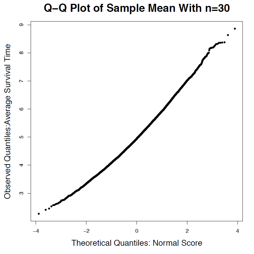Figure 6.7: Density and Normal Probability Plot of the Average Survival Time of n=2, 5, 30 Patients (Sample Mean). [Image Description (See Appendix D Figure 6.7)] Click on the image to enlarge it.

Here are the findings:

• The mean of the sample mean is 5, which equals the population mean regardless of the sample size n; the standard deviation roughly equals the population standard deviation divided by the square root of the sample size.
• The distribution of the sample mean inherits the right skewness of the parent population for relatively small sample sizes [latex]n = 2, 5[/latex], but it is roughly normal when [latex]n=30[/latex] (note that this trend towards normality increases as n grows beyond 30).

These two examples illustrate that the shape of the distribution of the sample mean [latex]\bar{X}[/latex] is approximately normal when the sample size n is sufficiently large, even if the population distribution is not normal. The more “non-normal” the parent population is, the larger n must be. This is the result of the central limit theorem, which will be discussed in the next section.