4.2 Probability Distribution of a Discrete Variable

1. Consider the chance experiment of flipping a balanced coin twice; the sample space is S = {HH, HT, TT, TH}. Let the random variable X = # of tails. Determine the probability distribution of X.
   • First, determine the possible values of $X$. If we flip a coin twice, we might observe zero tail (HH), one tail (HT, TH), and two tails (TT). Therefore, possible values are $x=0,1,2$.
   • Next, determine the probabilities $P(X=x),x=0,1,2$. Since the coin is balanced, it follows that $P(H)=P(T)=0.5$. Moreover, the two flips are independent, so the special multiplication rule applies. Thus,
     • $P(X=0)=P(HH)=P(H)\times P(H)=0.5\times 0.5=0.25$.
     • $P(X=1)=P(HT\text{ or }TH)=P(HT)+P(TH)=0.25+0.25=0.5$.
     • $P(X=2)=P(TT)=0.25$.

   Therefore, the probability distribution of X is

   Table 4.1: Probability Distribution of X=# of Heads

   $x$	0	1	2
   $P(X=x)$	0.25	0.5	0.25

   Note that the sum of the probabilities is one. That is

   $\begin{array}{rl}\sum P(X=x)& =P(X=0)+P(X=1)+P(X=2)\\ & =0.25+0.5+0.25=1.\end{array}$

2. A population consists of five students: Mark has no siblings, John has one sibling, both Rebecca and Sarah have two siblings, and Mary has three. Randomly pick one student and let $X$ be the number of siblings the student has. Determine the probability distribution of $X$.
   • First, observe that the possible values of $X$ are $x=0,1,2,3$
   • Next, determine the probabilities $P(X=x),x=0,1,2,3$. One student has no siblings, two students have two siblings, and one student has three siblings. Thus,
     • $P(X=0)=\frac{f}{N}=\frac{1}{5}=0.2$.
     • $P(X=1)=\frac{f}{N}=\frac{1}{5}=0.2$.
     • $P(X=2)=\frac{f}{N}=\frac{2}{5}=0.4$.
     • $P(X=3)=\frac{f}{N}=\frac{1}{5}=0.2$.

   The probability distribution of X is

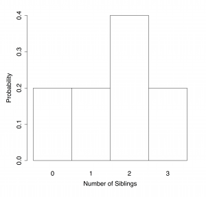
   Table 4.2: Probability Distribution of X=# of Siblings

Note that the sum of the probabilities is one. That is

$\begin{array}{rl}\sum P(X=x)& =P(X=0)+P(X=1)+P(X=2)+P(X=3)\\ & =0.2+0.2+0.4+0.2=1.\end{array}$

A probability distribution can also be represented as a histogram. Every possible value should have a separate bar for a discrete random variable.