There are two ways to quantify the extremeness of the data under the assumption that the null hypothesis [latex]H_0[/latex] is true: the critical value approach and the P-value approach. These two methods will give the same conclusion. For example, Bill claims he is not rich, and we want to prove that he is lying. The steps are:

1. Write down the hypotheses. [latex]H_0:[/latex] Bill is not rich versus [latex]H_a:[/latex] Bill is rich.
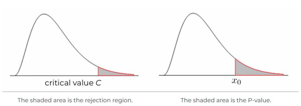
2. Collect the evidence and conclude. Suppose Bill has total wealth [latex]x_0[/latex], and we know the total wealth for every adult in the world; then we can draw the population distribution of the wealth, which is assumed to be the following graph.

1. 1. We can define the so-called rejection region by a cut-off C. Those with a total wealth at least C are defined as “rich” people, say the top 5%, meaning the shaded area (the left panel) is 0.05. Reject the null hypothesis [latex]H_0[/latex] if [latex]x_0[/latex] falls in the rejection region, i.e., [latex]x_0 \geq C[/latex], meaning Bill is one of those top 5% rich people. Note that the null hypothesis is [latex]H_0[/latex] Bill is not rich. Rejecting [latex]H_0[/latex] implies Bill is rich.
   2. We can also find the percentage of people at least as rich as Bill; that is the area to the right of [latex]x_0[/latex], the shaded area in the right panel. We call this area the P-value. We should reject the null hypothesis [latex]H_0[/latex] if the P-value is small. The smaller the area (P-value), the fewer people richer than Bill, the stronger the evidence that Bill is rich.

The shaded area is the rejection region.	The shaded area is the P-value.

Figure 8.3: Rejection Region (left panel) and P-value (right panel). [Image Description (See Appendix D Figure 8.3)]

8.4.1 The Critical Value Approach

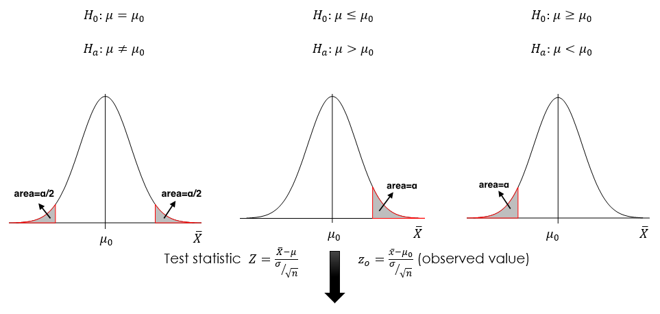
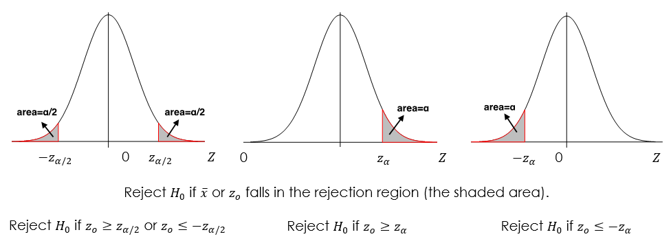
Recall that the main idea of hypothesis tests is to reject the null hypothesis [latex]H_0[/latex] if the sample mean [latex]\bar{x}[/latex] is too extreme, i.e., we should reject [latex]H_0[/latex] if [latex]\bar{x}[/latex] falls in the rejection region. If the population standard deviation [latex]\sigma[/latex] is known, the observed test statistic is [latex]z_o = \frac{\bar{x} - \mu_0}{\sigma / \sqrt{n}}[/latex]. If [latex]\bar{x}[/latex] is too extreme, the corresponding test statistic [latex]z_o[/latex] will also be too extreme. Since the standardized variable follows a standard normal distribution, we can use the standard normal density curve to define the rejection region. The key point for the critical value approach is that the total area of the rejection region equals the significance level of the test [latex]\alpha[/latex]. The values dividing the density curve into rejection and non-rejection regions are called the critical values, such as [latex]z_{\alpha}[/latex], [latex]z_{\alpha/2}[/latex], [latex]-z_{\alpha}[/latex], and [latex]-z_{\alpha/2}[/latex].

8.4.2 The P-value Approach

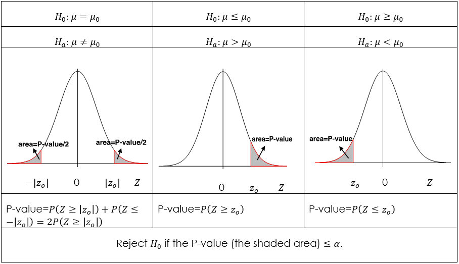
Another way to quantify the “extremeness” of the sample average is the P-value approach. We should reject the null [latex]H_0[/latex] if P-value [latex]\leq \alpha[/latex]. The P-value is the probability that the test statistic is at least as extreme as the observed statistic, given that the null hypothesis is true. The P-value is a measure of evidence against [latex]H_0[/latex] in favour of [latex]H_a[/latex]. The smaller the P-value, the stronger the evidence. A small P-value indicates that the observed value of the test statistic is very unlikely if the null is true. We should, therefore, reject the null hypothesis if the P-value [latex]\leq \alpha[/latex], where [latex]\alpha[/latex] is the significance level of the test. For example, if P-value=0.03, we reject the null if the significance level is [latex]\alpha = 0.1[/latex], or [latex]0.05[/latex] but not for [latex]\alpha = 0.01[/latex]. Here are some important facts about the P-value:

• P-value is a probability; therefore, it must be between 0 and 1.
• P-value is a conditional probability, given that the null [latex]H_0[/latex] is true. Note that the P-value is NOT the probability that the null is true, which is a common mistake.
• The P-value is a measure of evidence against [latex]H_0[/latex] in favour of [latex]H_a[/latex].
• Therefore, when performing a one-sided test, the direction of the inequality in the P-value calculation should be in the same direction as the inequality in the alternative [latex]H_a[/latex].
• The P-value of a two-sided test is twice that of a one-sided test with the same value of test statistic.

Calculation of the P-value: