Recall that a statistic is a function of the sample data. A statistic is an estimator when it is used to estimate the value of a population parameter. Each possible value of the estimator provides a point estimate of the parameter. For example, we use the sample mean [latex]\bar{X}[/latex] to estimate the population mean [latex]\mu[/latex]; therefore, [latex]\bar X[/latex] is an estimator of [latex]\mu[/latex]. Given a sample of size n, the value of the sample mean [latex]\bar{X}[/latex], denoted as [latex]\bar x[/latex], is a point estimate of the population parameter [latex]\mu[/latex]. Similarly, the sample standard deviation [latex]s[/latex] provides a point estimate of the population standard [latex]\sigma[/latex]. Recall that [latex]\bar{x}[/latex] and [latex]s[/latex] are numbers derived from the observed sample data and that different samples tend to yield different values of [latex]\bar{x}[/latex] and [latex]s[/latex].

Although a point estimate may give us an idea of the true value of the population parameter, the point estimate alone is insufficient. The value of a point estimate is usually not equal to the parameter of interest and error exists when estimating a parameter with a point estimate. In order to improve our estimation, we also need information about the precision of a point estimate, which is provided in the form of an interval (estimate − error, estimate + error). We call this kind of interval a confidence interval in the sense that by adjusting the error, we are able to claim that the parameter is within the interval with a certain confidence level.

7.1.1 One-Sample Z Interval When σ is Known

Recall the distribution of the sample mean [latex]\bar{X}[/latex]: for a normal population or a large sample size, the sample mean [latex]\bar{X} \sim N(\mu, \frac{\sigma}{\sqrt{n}})[/latex]. According to the 68.26-95.44-99.74 empirical rule for a normal distribution, 95.44% of the [latex]\bar{x}[/latex] values are within two standard deviations ([latex]2 \frac{\sigma}{\sqrt{n}}[/latex] ) away from the population mean [latex]\mu[/latex]. That is, 95.44% of the [latex]\bar{x}[/latex] values are within the interval [latex](\bar{x} - 2\frac{\sigma}{\sqrt{n}}, \bar{x} + 2\frac{\sigma}{\sqrt{n}})[/latex], if we consider all samples of size n. Therefore, for each of those [latex]\bar{x}[/latex] values, the distance between [latex]\bar{x}[/latex] and [latex]\mu[/latex] is at most [latex]2 \frac{\sigma}{\sqrt{n}}[/latex]. That is 95.44% of the [latex]\bar{x}[/latex] values satisfy

[latex]-2 \frac{\sigma}{\sqrt{n}}  <\bar{x} - \mu < 2 \frac{\sigma}{\sqrt{n}}.[/latex] In other words, 95.44% of the intervals in the form of [latex](\bar{x} - 2\frac{\sigma}{\sqrt{n}}, \bar{x} + 2\frac{\sigma}{\sqrt{n}})[/latex], contain the population mean [latex]\mu[/latex]. Similarly, 95% of the intervals in the form of [latex](\bar{x} - 1.96\frac{\sigma}{\sqrt{n}}, \bar{x} + 1.96\frac{\sigma}{\sqrt{n}}),[/latex] contain the population mean [latex]\mu[/latex]. We call the interval [latex](\bar{x} - 1.96\frac{\sigma}{\sqrt{n}}, \bar{x} + 1.96\frac{\sigma}{\sqrt{n}})[/latex]  a 95% confidence interval for [latex]\mu[/latex], which means we are 95% confident that the interval contains the population mean [latex]\mu[/latex]. In general, [latex](1 - \alpha ) \times 100\%[/latex] intervals in the form of [latex](\bar{x} - z_{\alpha/2}\frac{\sigma}{\sqrt{n}}, \bar{x} + z_{\alpha/2} \frac{\sigma}{\sqrt{n}})[/latex] contain the population mean [latex]\mu[/latex] and the interval [latex](\bar{x} - z_{\alpha/2}\frac{\sigma}{\sqrt{n}}, \bar{x} + z_{\alpha/2} \frac{\sigma}{\sqrt{n}})[/latex] is called a [latex](1 - \alpha) \times 100 \%[/latex] confidence interval. The number [latex](1 - \alpha) \times 100\%[/latex] is called the confidence level. Recall that [latex]z_{\alpha / 2}[/latex] is the z-score with area of [latex]\frac{\alpha}{2}[/latex] to its right. For example, suppose we wish to construct a 95% confidence interval for [latex]\mu[/latex], then [latex]1 - \alpha = 0.95 \Longrightarrow \alpha = 0.05 \Longrightarrow \frac{\alpha}{2} = 0.025 \Longrightarrow z_{\alpha /2} = z_{0.025} = 1.96.[/latex] Hence, a 95% confidence interval for [latex]\mu[/latex] is [latex](\bar{x} - 1.96\frac{\sigma}{\sqrt{n}}, \bar{x} + 1.96\frac{\sigma}{\sqrt{n}})[/latex].

7.1.2 Interpretation of a Confidence Interval

The interpretation of a confidence interval should be based on repeated samples. That is, suppose we repeatedly draw samples from the population of interest, and, for each sample, we calculate the confidence interval. If we continue this process indefinitely, then the confidence level is the relative frequency of intervals that contain the true value of the parameter of interest. For example, recall that the 95% Z-interval for [latex]\mu[/latex] is of the form [latex](\bar{x} - 1.96\frac{\sigma}{\sqrt{n}}, \bar{x} + 1.96\frac{\sigma}{\sqrt{n}})[/latex]; this means that 95% of such intervals contain the true value of [latex]\mu[/latex], while 5% of such intervals fail to capture [latex]\mu[/latex]. This is because [latex]\bar{X} \sim N(\mu, \frac{\sigma}{\sqrt{n}})[/latex], from which we are able to conclude that there is a 0.95 probability that the random variable [latex]\bar{X}[/latex] will be at most [latex]1.96 \frac{\sigma}{\sqrt{n}}[/latex] away from [latex]\mu[/latex]. However, once we obtain our random sample and compute the value of [latex]\bar{x}[/latex], it is no longer correct to say that there is a 0.95 probability the interval captures [latex]\mu[/latex]. Instead, we are 95% confident the interval captures [latex]\mu[/latex] (since 95% of all such intervals capture [latex]\mu[/latex], and we hope that the one we obtained is one of those 95% that contain [latex]\mu[/latex]).

Let’s consider an analogous example. If 95% of students will pass the final exam, then if we randomly choose a student, we should have 95% confidence that this student will pass the exam with the hope that he/she will be one of those 95% who pass the exam. Our confidence comes from the fact that 95% of students will pass the exam.

Example: Interpretation of Confidence Interval

Recall the beer example, wherein the population mean volume is [latex]\mu = 341[/latex] ml with a population standard deviation [latex]\sigma[/latex] = 5 ml.

1. Suppose we obtain a random sample of 100 bottles, from which we obtain a sample mean of [latex]\bar{x}[/latex] = 341.55. The 95% confidence interval is:
   [latex](\bar{x} - 1.96\frac{\sigma}{\sqrt{n}}, \bar{x} + 1.96\frac{\sigma}{\sqrt{n}}) = (341.55 - 1.96 \frac{5}{\sqrt{100}}, 341.55 + 1.96 \frac{5}{\sqrt{100}}) = (340.57,  342.53 ).[/latex]
   The population mean, [latex]\mu=341[/latex], is within the interval since the sample mean (red diamond) is within 1.96 standard deviations of [latex]\mu[/latex] (blue lines).
2. We repeat the previous step 20 times and observe that only one sample mean is outside the blue lines and hence, only one interval does not contain [latex]\mu[/latex]; the other nineteen intervals all contain [latex]\mu[/latex], which is 95% out of 20.
3. For each interval, we hope it is one of those 95% contain [latex]\mu[/latex]. Therefore, we have 95% confidence that each of those intervals contains the population mean [latex]\mu=341[/latex].

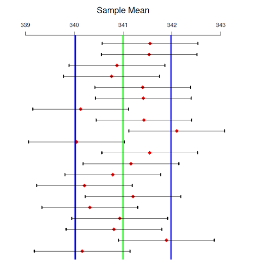
Note: In the above example, there is no guarantee that exactly 95% of the samples will capture [latex]\mu[/latex], but rather, this is the expected percentage. As we obtain more samples, the percentage of intervals containing [latex]\mu[/latex] will converge to 95%.

Example: Interpretation of One-sample Z Interval

A machine fills beer into bottles whose volume is supposed to be 341 ml, but the exact amount varies from bottle to bottle. We randomly pick 100 bottles and obtain the sample mean volume is 339 ml. Assume the population standard deviation [latex]\sigma[/latex] = 5 ml. A 95% confidence interval for the population mean volume [latex]\mu[/latex] is

[latex]\begin{align*} &(\bar{x} - z_{\alpha /2}\frac{\sigma}{\sqrt{n}}, \bar{x} +z_{\alpha /2}\frac{\sigma}{\sqrt{n}}) \\ &= 339 \pm 1.96 \times \frac{5}{\sqrt{100}} \\ &= (399 - 0.98, 339 + 0.98) \\ &= (338.02, 339.98).\end{align*}[/latex]

Interpret this interval. Does it provide evidence to suggest the machine is not working properly?

Interpretation: We are 95% confident that the interval (338.02, 339.98) contains the population mean volume [latex]\mu[/latex]. In other words, we are 95% confident that the population mean volume [latex]\mu[/latex] is somewhere between 338.02 ml and 339.98 ml.

Since the interval does not contain 341, we are 95% confident that the true mean [latex]\mu[/latex] is not equal to 341 ml. As a result, we have evidence to suggest that the machine is NOT working properly. Moreover, since the entire interval is below 341 ml, the data provide evidence that the true mean volume [latex]\mu[/latex] is less than 341 ml.

Note: The population mean [latex]\mu[/latex] is a constant; however, we don’t know its value. It can be anywhere within the interval or outside the interval. We are 95% confident that [latex]\mu[/latex] is within the resulting confidence interval.

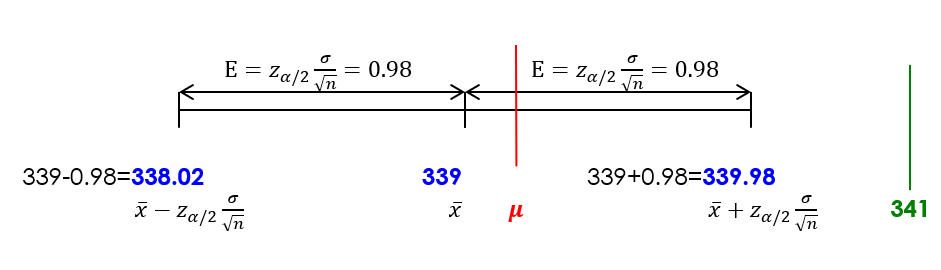
7.1.3 Margin of Error and Sample Size Calculation

The length of a confidence interval [latex](\bar{x} - z_{\frac{\alpha}{2}} \frac{\sigma}{\sqrt{n}}, \bar{x} + z_{\frac{\alpha}{2}} \frac{\sigma}{\sqrt{n}})[/latex] is twice of the quantity [latex]z_{\frac{\alpha}{2}} \frac{\sigma}{\sqrt{n}}[/latex]. The term [latex]z_{\frac{\alpha}{2}} \frac{\sigma}{\sqrt{n}}[/latex] is called the margin of error, denoted as [latex]E[/latex] and it quantifies the accuracy/precision of an estimate. The margin of error is the largest distance between the estimate [latex]\bar{x}[/latex] and the parameter [latex]\mu[/latex] given a certain confidence level. Figure 7.2 implies that a confidence interval’s length equals twice the margin of error. The larger the margin of error, the wider the confidence interval is, and hence, the more confident we are that the interval contains the parameter of interest, but the estimate is less precise. This is the trade-off between confidence level and precision. If we would like to have a higher level of precision, we have to reduce the confidence level and, therefore, reduce the length of the interval. The formula of the margin of error (i.e., [latex]E = z_{\alpha /2 } \frac{\sigma}{\sqrt{n}}[/latex]) implies that three things affect the margin of error: the confidence level [latex]1-\alpha[/latex], the population standard deviation, and the sample size [latex]n[/latex]. If we want to improve precision (i.e., reduce the margin of error [latex]E[/latex]) and maintain the same level of confidence (i.e., fix [latex]1 - \alpha[/latex] or [latex]\alpha[/latex] and hence the z–score [latex]z_{\alpha / 2}[/latex] ), we have to increase the sample size n.

It is often useful to know the minimum sample size n needed in order to ensure the margin is at most [latex]E[/latex] when estimating the population mean [latex]\mu[/latex] with the sample mean [latex]\bar{x}[/latex]. More specifically, suppose we have a fixed confidence level [latex]1 - \alpha[/latex], and we want the margin of error to be at most [latex]E[/latex]. Then, recalling that margin of error is defined as [latex]E = z_{\alpha /2} \frac{\sigma}{\sqrt{n}}[/latex], we solve for n in order to obtain:

[latex]n = \left( \frac{\sigma \times z_{\alpha / 2}}{E} \right)^2.[/latex]

Since the sample size is an integer, we should round the final result up to the next integer (rounding down will give us a margin of error that is slightly larger than [latex]E[/latex], while rounding up will give us a margin of error that is slightly smaller than [latex]E[/latex]).