6.6 Assignment 6

Purposes

This assignment has two parts to assess your knowledge of the distribution of the sample mean (including the mean, standard deviation, and shape) and the central limit theorem.

Instructions

Part A

Complete the following:

1. Explain the relationship between the population mean [latex]\mu[/latex], sample mean [latex]\bar{X}[/latex], and a value of the sample mean [latex]\bar{x}[/latex]. Which is the population parameter, which is an estimate, and which is an estimator? (5 marks: 3+2)
2. Explain in plain English why the standard deviation of the sample mean [latex]\sigma_{\bar{X}}[/latex] becomes smaller when the sample size increases. (2 marks)
3. Does the sample size [latex]n[/latex] affect the mean of all possible sample means? Explain your answer. (3 marks)
4. Does the sample size [latex]n[/latex] affect the standard deviation of all possible sample means? Explain your answer. (3 marks)
5. What does the central limit theorem tell us? (3 marks)
6. Do we need the population to be normal or the sample size [latex]n[/latex] to be large to claim that [latex]\mu_{\scriptsize \bar{X}} = \mu[/latex] and [latex]\sigma_{\scriptsize \bar{X}} = \frac{\sigma}{\sqrt{n}}[/latex]? Explain your answer. (3 marks)
7. Suppose that [latex]X[/latex], the rent of a one-bedroom apartment in Edmonton, follows a distribution with a mean of $700 and a standard deviation of $400. Its density curve is given below.
   

   

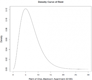
   1. Describe the population distribution of the rent of a one-bedroom apartment in Edmonton, i.e., the distribution of [latex]X[/latex]. Comment on modality, centre, spread, and shape. (3 marks)
   2. If you randomly pick four one-bedroom apartments, describe the sampling distribution of their average rent. Indicate the mean, standard deviation, and shape. (3 marks)
   3. If you randomly pick 100 one-bedroom apartments, describe the sampling distribution of their average rent. Indicate the mean, standard deviation, and shape. (3 marks)
   4. If you randomly pick 100 one-bedroom apartments, find the probability that their average rent is above $800. (4 marks)
   5. Fill in the following table about the mean, the standard deviation, and the shape of [latex]X[/latex] (the variable of interest, the population) and the sample mean [latex]\bar{X}[/latex] with different sample size [latex]n[/latex]. (4 marks)
      

      Variable	Mean	Standard Deviation	Shape
      [latex]X[/latex] (population)	[latex]\mu =[/latex]	[latex]\sigma =[/latex]	Not normal, right skewed
      [latex]\bar{X}[/latex] with [latex]n = 4[/latex]	[latex]\mu_{\scriptsize \bar{X}} = \mu =[/latex]	[latex]\sigma_{\scriptsize \bar{X}} = \frac{\sigma}{\sqrt{n}} =[/latex]
      [latex]\bar{X}[/latex] with [latex]n = 100[/latex]	[latex]\mu_{\scriptsize \bar{X}} = \mu =[/latex]	[latex]\sigma_{\scriptsize \bar{X}} = \frac{\sigma}{\sqrt{n}} =[/latex]

Part B

Finish the following questions using R and R commander. Make sure that you copy and paste the computer outputs into the space below each question, and write down your answers in statements.

1. Use R commander to explore the distribution of the sample mean [latex]\bar{X}[/latex] when the variable of interest [latex]X[/latex] follows a normal distribution.
   1. Generate 1,000 observations from a normal distribution with a mean of 70 and a standard deviation of 10. Set the random number seed to be 6,194. Draw a histogram, box plot, and a normal probability plot on these 1,000 observations. Comment on the centre, spread (variation), and shape of the distribution. We call this the population distribution, i.e., the distribution of [latex]X\sim N(70,\ 10)[/latex]. (6 marks)
   2. Generate [latex]n = 2[/latex] observations from a normal distribution with a mean of 70 and standard deviation of 10, and calculate the mean of these two observations. Repeat this procedure 500 times. Draw a histogram, box plot, and normal probability plot on these 500 sample means, comment on the centre, spread (variation), and shape of the distribution. We call this the sampling distribution of the sample mean [latex]\bar{X}[/latex] with sample size [latex]n = 2[/latex]. (6 marks)
   3. Repeat part (b) with [latex]n = 10[/latex] to obtain the sampling distribution of the sample mean [latex]\bar{X}[/latex] with sample size [latex]n = 10[/latex]. (6 marks)
   4. Repeat part (b) with [latex]n = 36[/latex] to obtain the sampling distribution of the sample mean [latex]\bar{X}[/latex] with sample size [latex]n = 36[/latex]. (6 marks)
   5. Complete the following table about the mean, the standard deviation, and the shape of [latex]X[/latex] (the variable of interest, the population) and the sample mean [latex]\bar{X}[/latex] with different sample size [latex]n[/latex]. (6 marks)
      

      Variable	Mean	Standard Deviation	Shape
      [latex]X[/latex] (population)	[latex]\mu =[/latex]	[latex]\sigma =[/latex]	Normal
      [latex]\bar{X}[/latex] with [latex]n = 2[/latex]	[latex]\mu_{\scriptsize \bar{X}} = \mu =[/latex]	[latex]\sigma_{\scriptsize \bar{X}} = \frac{\sigma}{\sqrt{n}} =[/latex]
      [latex]\bar{X}[/latex] with [latex]n = 10[/latex]	[latex]\mu_{\scriptsize \bar{X}} = \mu =[/latex]	[latex]\sigma_{\scriptsize \bar{X}} = \frac{\sigma}{\sqrt{n}} =[/latex]
      [latex]\bar{X}[/latex] with [latex]n = 36[/latex]	[latex]\mu_{\scriptsize \bar{X}} = \mu =[/latex]	[latex]\sigma_{\scriptsize \bar{X}} = \frac{\sigma}{\sqrt{n}} =[/latex]

2. Use R commander to explore the distribution of the sample mean [latex]\bar{X}[/latex] when the variable of interest [latex]X[/latex] follows an extremely skewed distribution.
   1. Generate 1,000 observations from an exponential distribution with mean 5 (or rate = 1/5 = 0.2). Set the random number seed to be 4,067. Draw a histogram, box plot, and a normal probability plot on these 1,000 observations. Comment on the centre, spread (variation), and shape of the distribution. We call this the population distribution, i.e., the distribution of [latex]X\sim Exponential(5)[/latex]. Note that the standard deviation of an exponential distribution is the same as the mean, i.e., [latex]\sigma = \mu = 5[/latex] in this question. (6 marks)
   2. Generate [latex]n = 2[/latex] observations from an exponential distribution with mean 5, and calculate the mean of these two observations. Repeat this procedure 500 times. Draw a histogram, box plot, and a normal probability plot on these 500 sample means, comment on the centre, spread (variation), and shape of the distribution. We call this the sampling distribution of the sample mean [latex]\bar{X}[/latex] with sample size [latex]n = 2[/latex]. (6 marks)
   3. Repeat part (b) with [latex]n = 10[/latex] to obtain the sampling distribution of the sample mean [latex]\bar{X}[/latex] with sample size [latex]n = 10[/latex]. (6 marks)
   4. Repeat part (b) with [latex]n = 36[/latex] to obtain the sampling distribution of the sample mean [latex]\bar{X}[/latex] with sample size [latex]n = 36[/latex]. (6 marks)
   5. Complete the following table about the mean, the standard deviation, and the shape of [latex]X[/latex] (the variable of interest, the population) and the sample mean [latex]\bar{X}[/latex] with different sample size [latex]n[/latex]. (6 marks)
      

      Variable	Mean	Standard Deviation	Shape
      [latex]X[/latex] (population)	[latex]\mu =[/latex]	[latex]\sigma =[/latex]	Not normal, right skewed
      [latex]\bar{X}[/latex] with [latex]n = 2[/latex]	[latex]\mu_{\scriptsize \bar{X}} = \mu =[/latex]	[latex]\sigma_{\scriptsize \bar{X}} = \frac{\sigma}{\sqrt{n}} =[/latex]
      [latex]\bar{X}[/latex] with [latex]n = 10[/latex]	[latex]\mu_{\scriptsize \bar{X}} = \mu =[/latex]	[latex]\sigma_{\scriptsize \bar{X}} = \frac{\sigma}{\sqrt{n}} =[/latex]
      [latex]\bar{X}[/latex] with [latex]n = 36[/latex]	[latex]\mu_{\scriptsize \bar{X}} = \mu =[/latex]	[latex]\sigma_{\scriptsize \bar{X}} = \frac{\sigma}{\sqrt{n}} =[/latex]