13.8 Inferences for the Parameters in SLRM
There are three population parameters in the simple regression model (SLRM): the population intercept [latex]\beta_0[/latex], the population slope [latex]\beta_1[/latex] , and the standard deviation of the error [latex]\sigma[/latex]. The three population parameters can be estimated by the least-squares estimates:
- [latex]b_0 = \bar{y} - b_1 \bar{x}[/latex] estimates the population intercept [latex]\beta_0[/latex];
- [latex]b_1 = \frac{S_{xy}}{S_{xx}}[/latex] estimates the population intercept [latex]\beta_1[/latex];
- the sample standard deviation of the residuals [latex]s_e = \sqrt{\frac{\sum (e_i - \bar{e})^2}{n-2}} = \sqrt{\frac{\sum e_i^2}{n-2}} = \sqrt{\frac{SSE}{n-2}}[/latex] estimates the standard deviation of the error term [latex]\sigma[/latex], where [latex]SSE = SST - SSR = SST - r^2 SST = S_{yy} - \frac{S_{xy}^2}{S_{xx} S_{yy}} S_{yy} = S_{yy} - b_1 S_{xy}[/latex].
We are especially interested in testing whether the slope parameter [latex]\beta_1[/latex] differs from 0. If [latex]\beta_1 = 0[/latex], the predictor variable [latex]x[/latex] provides no information about the conditional mean of [latex]Y[/latex], and hence there is no point fitting a regression model. Inferences about [latex]\beta_1[/latex] are based on the distribution of the least-squares slope [latex]b_1[/latex].
13.8.1 Distribution of the Least-squares Slope b1
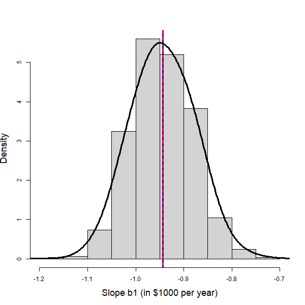
In the previous example, a least-squares regression line was developed to predict the price of used cars with their ages; using a sample of 15 used cars, the fitted line had a slope of [latex]b_1 = -0.9432[/latex]. Does [latex]b_1 = -0.9432[/latex] provide evidence of a linear association between the price and age of all used cars? In order to answer this question, we need a better understanding of the distribution of [latex]b_1[/latex]. Suppose, for example, that we repeat this experiment 1000 times by obtaining 1000 samples of 15 used cars, fitting 1000 regression lines, and as such, getting 1000 different values of [latex]b_1[/latex], each of which is a point estimate of the population slope [latex]\beta_1[/latex]. The distribution of these 1000 values of [latex]b_1[/latex], therefore, provides an estimate of the true distribution of all such [latex]b_1[/latex]. The following histogram illustrates the distribution of 1000 values of [latex]b_1[/latex].
 |
It can be shown that the distribution of [latex]b_1[/latex] is normal with
That is [latex]b_1 \sim N(\beta_1, \frac{\sigma}{\sqrt{S_{xx}}})[/latex]. Thus, we can standardize [latex]b_1[/latex] in order to obtain: [latex]\frac{b_1 - \beta_1}{\frac{\sigma}{\sqrt{S_{xx}}}} \sim N(0, 1)[/latex]. When the standard deviation of the error term [latex]\sigma[/latex] is unknown, it can be estimated by the standard deviation of the residuals [latex]s_e[/latex]. This leads to the studentized variable [latex]\frac{b_1 - \beta_1}{\frac{s_e}{\sqrt{S_{xx}}}} \sim t \text{ distribution with } df = n-2[/latex]. |
Hence, inferences about the slope parameter [latex]\beta_1[/latex] are based on a [latex]t[/latex] distribution with degrees of freedom [latex]n-2[/latex]. Note that we lose two degrees of freedom in finding [latex]b_0[/latex] and [latex]b_1[/latex].
13.8.2 t Test and t Interval for the Slope Parameter β1
Assumptions:
- The response variable (or the error term) is normally distributed.
- The standard deviation of the response variable (or error term) is the same for all values of the predictor variable.
- The observations are independent.
- The data come from a simple random sample.
Steps to perform a test on the slope parameter [latex]\beta_1[/latex]:
- Set up the hypotheses:
The predictor is usefulpositive associationnegative association[latex]H_0: \beta_1 = 0[/latex][latex]H_0: \beta_1 \leq 0[/latex][latex]H_0: \beta_1 \geq 0[/latex][latex]H_a: \beta_1 \neq 0[/latex][latex]H_a: \beta_1 > 0[/latex][latex]H_a: \beta_1 < 0[/latex]
- State the significance level [latex]\alpha[/latex].
- Compute the test statistic: [latex]t_o = \frac{b_1}{\frac{s_e}{\sqrt{S_{xx}}}}[/latex] with degree of freedom [latex]df = n-2[/latex].
- Find the P-value or rejection region
The predictor is usefulpositive associationnegative association
Null [latex]H_0: \beta_1 = 0[/latex][latex]H_0: \beta_1 \leq 0[/latex][latex]H_0: \beta_1 \geq 0[/latex]Alternative [latex]H_a: \beta_1 \neq 0[/latex][latex]H_a: \beta_1 > 0[/latex][latex]H_a: \beta_1 < 0[/latex]P-value [latex]2P(t \geq |t_o|)[/latex][latex]P(t \geq t_o)[/latex][latex]P(t \leq t_o)[/latex]Rejection region [latex]t \geq t_{\alpha /2}[/latex] or [latex]t \leq - t_{\alpha /2}[/latex] [latex]t \geq t_{\alpha}[/latex][latex]t \leq - t_{\alpha}[/latex] - Reject the null [latex]H_0[/latex] if P-value [latex]\leq \alpha[/latex] or [latex]t_o[/latex] falls in the rejection region.
- Conclusion.
The [latex](1 - \alpha) \times 100\%[/latex] [latex]t[/latex] confidence interval for [latex]\beta_1[/latex] corresponding to the [latex]t[/latex] test:
| The predictor is useful | positive association | negative association | |
|---|---|---|---|
| Null | [latex]H_0: \beta_1 = 0[/latex] | [latex]H_0: \beta_1 \leq 0[/latex] | [latex]H_0: \beta_1 \geq 0[/latex] |
| Alternative | [latex]H_a: \beta_1 \neq 0[/latex] | [latex]H_a: \beta_1 > 0[/latex] | [latex]H_a: \beta_1 < 0[/latex] |
| CI | [latex]\left( b_1 - t_{\alpha / 2} \frac{s_e}{\sqrt{S_{xx}}}, b_1 + t_{\alpha / 2} \frac{s_e}{\sqrt{S_{xx}}} \right)[/latex] | [latex](b_1 - t_{\alpha} \frac{s_e}{\sqrt{S_{xx}}}, \infty )[/latex] | [latex]( - \infty , b_1 + t_{\alpha} \frac{s_e}{\sqrt{S_{xx}}} )[/latex] |
| Decision | Reject [latex]H_0[/latex] if the interval does not contain 0. | ||
Example: t-Test and t Interval for the Slope Parameter [latex]\color{white}{\beta_1}[/latex]
Recall the used car example. We have the summaries
[latex]n = 15, \sum x_i = 92, \sum x_i^2 = 724, \sum y_i = 125, \sum y_i^2 = 1193, \sum x_i y_i = 616[/latex].
We can calculate:
[latex]\begin{align*}S_{xy} &= \sum x_i y_i - \frac{\left( \sum x_i \right) \left( \sum y_i \right) }{n} = 616 - \frac{92 \times 125}{15} = -150.667,\\S_{xx} &= \sum x_i^2 - \frac{ \left( \sum x_i\right)^2 }{n} = 724 - \frac{92^2}{15} = 159.733,\\S_{yy} &= \sum y_i^2 - \frac{ \left( \sum y_i \right)^2 }{n} = 1193 - \frac{125^2}{15} = 151.333.\end{align*}[/latex]
[latex]\begin{align*}b_1 &= \frac{S_{xy}}{S_{xx}} = \frac{-150.667}{159.733} = -0.9432; \\b_0&=\bar y-b_1\bar x=\frac{\sum y_i}{n}-b_1 \frac{\sum x_i}{n}=\frac{125}{15}-(-0.9432) \frac{92}{15}=14.118.\end{align*}[/latex]
And the least-square straight line is [latex]\widehat{\text{price}} = 14.118 - 0.9432 \times \text{age}[/latex].
- Test at the 5% significance level whether age is a useful predictor for the price of a used car.
Steps:- Set up the hypotheses. [latex]H_0: \beta_1 = 0[/latex] versus [latex]H_a: \beta_1 \neq 0[/latex].
- The significance level is [latex]\alpha = 0.05[/latex].
- Compute the value of the test statistic: [latex]t_o = \frac{b_1}{\frac{s_e}{\sqrt{S_{xx}}}}[/latex] with [latex]df = n -2.[/latex] First, [latex]SSE = S_{yy} - b_1 S_{xy} = 151.333 - (-0.9432) \times (-150.667) = 9.224[/latex] so that [latex]s_e = \sqrt{\frac{SSE}{n-2}} = \sqrt{\frac{9.224}{13}} = 0.842[/latex]. Therefore,
[latex]t_o = \frac{b_1}{\frac{s_e}{\sqrt{S_{xx}}}} = \frac{-0.9432}{\left( \frac{0.842}{\sqrt{159.733}} \right)} = -14.158, df = n-2 = 15-2 = 13[/latex].
- Find the P-value. For a two-tailed test with [latex]df=13[/latex],
P-value [latex]=2P(t \geq |t_o|) = 2P(t \geq 14.158) < 2 \times 0.0005 = 0.001[/latex], since [latex]t_{0.0005} = 4.221.[/latex] - Decision: Reject the null [latex]H_0[/latex] since P-value [latex]< 0.001 < 0.05 (\alpha).[/latex]
- Conclusion. At the 5% significance level, we have sufficient evidence that age is a useful predictor of the price of a used car.
- Obtain a [latex]t[/latex] confidence interval for the slope parameter [latex]\beta_1[/latex] corresponding to the test in part (a).
A 95% two-tailed interval corresponds to a two-tailed test at the 5% significance level. Therefore, since[latex]df = 13, \alpha = 0.05[/latex], and [latex]t_{\alpha / 2} = t_{0.025} = 2.160[/latex]
It follows that a 95% confidence interval for [latex]\beta_1[/latex] is:
[latex]b_1 \pm t_{\alpha / 2} \frac{s_e}{\sqrt{S_{xx}}} = (-0.9432) \pm 2.160 \times \frac{0.842}{\sqrt{159.733}} = (-1.087, -0.799)[/latex].
- Interpret the interval. Does it support the conclusions of the hypothesis test in part (a)?
We are 95% confident that [latex]\beta_1[/latex] is somewhere between -1.087 and -0.799 ($1000 per year). Hence, we estimate that the mean price of used cars drops from $799 to $1087 when they get one year older.
Yes, it supports the conclusions of the hypothesis test in part (a). The interval does not contain 0; which implies [latex]\beta_1 \neq 0[/latex] with 95% confidence. Therefore, the interval suggests age is a useful predictor for the price of used cars, which is the conclusion of the test in part (a).
