9.3 Paired t Test and Interval Based on Paired Sample
Two samples are considered paired if each observation in the first sample is related to exactly one observation in the second sample and each observation in the second sample is related to exactly one observation in the first sample. Some examples of paired observations include:
- Reaction times of an individual before and after consuming caffeine.
- The weight of a patient before and after a medical treatment.
- The fuel consumption of the same vehicle when it is driven at two different speeds.
- The ages of a husband and wife in the same marriage.
Example: Independent Sample or Paired Sample?
- We randomly selected 40 males and 40 females and compared the average time they spent watching TV. Is this an independent sample or a paired sample?
An independent sample since there is no relationship between those 40 males and 40 females. - We randomly selected 40 couples and compared the time the husbands and wives spent watching TV. Is this an independent sample or a paired sample?
Paired sample, since those 40 males and 40 females are husbands and wives from the same households. - This table shows men's and women's winning times (in minutes) in the New York City Marathon between 1978 and 2006 (www.nycmarathon.org). Is this an independent sample or a paired sample?
Table 9.2: Winning Times for Men and Women of New York City Marathon 1978-2006
| Year | Men | Women | Difference | Year | Men | Women | Difference |
| 1978 | 132.2 | 152.5 | 20.3 | 1993 | 130.1 | 146.4 | 16.3 |
| 1979 | 131.7 | 147.6 | 15.9 | 1994 | 131.4 | 147.6 | 16.2 |
| 1980 | 129.7 | 145.7 | 16.0 | 1995 | 131 | 148.1 | 17.1 |
| 1981 | 128.2 | 145.5 | 17.3 | 1996 | 129.9 | 148.3 | 18.4 |
| 1982 | 129.5 | 147.2 | 17.7 | 1997 | 128.2 | 148.7 | 20.5 |
| 1983 | 129 | 147 | 18.0 | 1998 | 128.8 | 145.3 | 16.5 |
| 1984 | 134.9 | 149.5 | 14.6 | 1999 | 129.2 | 145.1 | 15.9 |
| 1985 | 131.6 | 148.6 | 17.0 | 2000 | 130.2 | 145.8 | 15.6 |
| 1986 | 131.1 | 148.1 | 17.0 | 2001 | 127.7 | 144.4 | 16.7 |
| 1987 | 131 | 150.3 | 19.3 | 2002 | 128.1 | 145.9 | 17.8 |
| 1988 | 128.3 | 148.1 | 19.8 | 2003 | 130.5 | 142.5 | 12.0 |
| 1989 | 128 | 145.5 | 17.5 | 2004 | 129.5 | 143.2 | 13.7 |
| 1990 | 132.7 | 150.8 | 18.1 | 2005 | 129.5 | 144.7 | 15.2 |
| 1991 | 129.5 | 147.5 | 18.0 | 2006 | 130 | 145.1 | 15.1 |
| 1992 | 129.5 | 144.7 | 15.2 |
Paired sample since the winning times for men and women in the same year were compared. We should not compare the winning time for men in 2006 with the winning time for women in 2000 since the weather conditions vary from year to year, affecting the winning time.
A paired t-test and a paired t-interval are exactly a one-sample t-test and a one-sample t-interval on the paired differences. Therefore, the assumptions and the procedures for a paired t-test are the same as those for a one-sample t-test.
Assumptions:
- The sample of paired differences [latex]d_i, i = 1, \dots, n[/latex] is a simple random sample (SRS) from the population of all possible paired differences.
- The paired differences follow a normal distribution or a large number of paired differences [latex](n \geq 30)[/latex].
Steps:
- Set up the hypotheses:
Two-tailedRight-tailedLeft-tailed[latex]H_0: \mu_1 - \mu_2 = \delta_0[/latex][latex]H_0: \mu_1 - \mu_2 \leq \delta_0[/latex][latex]H_0: \mu_1 - \mu_2 \geq \delta_0[/latex][latex]H_a: \mu_1 - \mu_2 \neq \delta_0[/latex][latex]H_a: \mu_1 - \mu_2 \: \gt \: \delta_0[/latex][latex]H_a: \mu_1 - \mu_2 \: \lt \: \delta_0[/latex]
Note: [latex]\delta_0[/latex] can be any value tested, but in most cases [latex]\delta_0 = 0[/latex]. Some textbooks state the hypotheses using [latex]\mu_d = \mu_1 - \mu_2[/latex].
- State the significance level [latex]\alpha[/latex].
- Compute the value of the test statistic: [latex]t_o = \frac{\bar{d} - \delta_0}{s_d / \sqrt{n}}[/latex], with degrees of freedom [latex]df= n-1[/latex], where n is the number of paired differences and the mean and standard deviation of the paired differences are given by
[latex]\bar{d} = \frac{\sum d_i}{n}, s_d = \sqrt{\frac{(\sum d_i^2) - \frac{(\sum d_i)^2}{n}}{n-1}}.[/latex]
- Use the t-score table (Table IV) to find the P-value or rejection region.
Two-tailedRight-tailedLeft-tailed
Null [latex]H_0: \mu_1 - \mu_2 = \delta_0[/latex][latex]H_0: \mu_1 - \mu_2 \leq \delta_0[/latex][latex]H_0: \mu_1 - \mu_2 \geq \delta_0[/latex]Alternative [latex]H_a: \mu_1 - \mu_2 \neq \delta_0[/latex][latex]H_a: \mu_1 - \mu_2 \: \gt \: \delta_0[/latex][latex]H_a: \mu_1 - \mu_2 \: \lt \: \delta_0[/latex]P-value [latex]2P(t \geq |t_o|)[/latex][latex]P(t \geq t_o)[/latex][latex]P(t \leq t_o)[/latex]Rejection region [latex]t \geq t_{\alpha / 2}[/latex] or [latex]t \leq - t_{\alpha / 2}[/latex] [latex]t \geq t_{\alpha}[/latex][latex]t \leq - t_{\alpha}[/latex] - Reject the null [latex]H_0[/latex] if P-value [latex]\leq \alpha[/latex] or [latex]t_o[/latex] falls in the rejection region.
- Conclusion.
A [latex](1 – \alpha) \times 100\%[/latex] confidence interval for [latex]\mu_d = \mu_1 - \mu_2[/latex] corresponding to a hypothesis test at the significance level [latex]\alpha[/latex] is
|
Two-tailed
|
Right-tailed
|
Left-tailed
|
|
|---|---|---|---|
| Null |
[latex]H_0: \mu_1 - \mu_2 = \delta_0[/latex]
|
[latex]H_0: \mu_1 - \mu_2 \leq \delta_0[/latex]
|
[latex]H_0: \mu_1 - \mu_2 \geq \delta_0[/latex]
|
| Alternative |
[latex]H_a: \mu_1 - \mu_2 \neq \delta_0[/latex]
|
[latex]H_a: \mu_1 - \mu_2 \: \gt \: \delta_0[/latex]
|
[latex]H_a: \mu_1 - \mu_2 \: \lt \: \delta_0[/latex]
|
| [latex](1 – \alpha) \times 100\%[/latex] CI |
[latex](\bar{d} - t_{\alpha / 2} \frac{s_d}{\sqrt{n}}, \bar{d} + t_{\alpha / 2} \frac{s_d}{\sqrt{n}})[/latex]
|
[latex](\bar{d} - t_{\alpha} \frac{s_d}{\sqrt{n}}, \infty)[/latex]
|
[latex](- \infty, \bar{d} + t_{\alpha} \frac{s_d}{\sqrt{n}})[/latex]
|
| Decision | Reject [latex]H_0[/latex] if [latex]\delta_0[/latex] is outside the interval | ||
Example: Paired t-test and Paired t-interval
This table shows men and women's winning times (in minutes) in the New York City Marathon between 1978 and 2006.
| Year | Men | Women | Difference | Year | Men | Women | Difference |
| 1978 | 132.2 | 152.5 | 20.3 | 1993 | 130.1 | 146.4 | 16.3 |
| 1979 | 131.7 | 147.6 | 15.9 | 1994 | 131.4 | 147.6 | 16.2 |
| 1980 | 129.7 | 145.7 | 16.0 | 1995 | 131 | 148.1 | 17.1 |
| 1981 | 128.2 | 145.5 | 17.3 | 1996 | 129.9 | 148.3 | 18.4 |
| 1982 | 129.5 | 147.2 | 17.7 | 1997 | 128.2 | 148.7 | 20.5 |
| 1983 | 129 | 147 | 18.0 | 1998 | 128.8 | 145.3 | 16.5 |
| 1984 | 134.9 | 149.5 | 14.6 | 1999 | 129.2 | 145.1 | 15.9 |
| 1985 | 131.6 | 148.6 | 17.0 | 2000 | 130.2 | 145.8 | 15.6 |
| 1986 | 131.1 | 148.1 | 17.0 | 2001 | 127.7 | 144.4 | 16.7 |
| 1987 | 131 | 150.3 | 19.3 | 2002 | 128.1 | 145.9 | 17.8 |
| 1988 | 128.3 | 148.1 | 19.8 | 2003 | 130.5 | 142.5 | 12.0 |
| 1989 | 128 | 145.5 | 17.5 | 2004 | 129.5 | 143.2 | 13.7 |
| 1990 | 132.7 | 150.8 | 18.1 | 2005 | 129.5 | 144.7 | 15.2 |
| 1991 | 129.5 | 147.5 | 18.0 | 2006 | 130 | 145.1 | 15.1 |
| 1992 | 129.5 | 144.7 | 15.2 |
- At the 1% significance level, do the data provide sufficient evidence that, there is a difference in mean winning times between males and females? Note that the sample mean and standard deviation of the paired differences are [latex]\bar{d} = 16.85[/latex] and [latex]s_d = 1.98[/latex] respectively.
Steps:- Set up the hypotheses: [latex]H_0: \mu_{\scriptsize F} - \mu_{\scriptsize M} = 0[/latex] versus [latex]H_a: \mu_{\scriptsize F} - \mu_{\scriptsize M} \neq 0[/latex].
- The significance level is [latex]\alpha = 0.01[/latex].
- Compute the value of the test statistic: [latex]t_o = \frac{\bar{d} - \delta_0}{s_d / \sqrt{n}} = \frac{16.85 - 0}{1.98 / \sqrt{29}} = 45.828[/latex] with [latex]df = n-1 = 29 -1 = 28[/latex].
- Find the P-value. For a two-tailed test, the P-value is twice the area to the right of the absolute value of the observed test statistic [latex]t_o[/latex].
P-value = [latex]2P(t \geq |t_o|) = 2P(t \geq 45.828) < 2 \times 0.0005=0.001[/latex], since [latex]45.828 \: \gt \: 3.674 (t_{0.0005})[/latex] - Decision: Since the P- value [latex]< 0.001<0.01(\alpha)[/latex], we reject the null hypothesis [latex]H_0[/latex].
- Conclusion: At the 1% significance level, the data provide sufficient evidence that there is a difference in mean winning times between males and females.
- Obtain a 99% two-tailed interval for the difference in mean winning times between males and females, i.e., [latex]\mu_{\scriptsize F}-\mu_{\scriptsize M}[/latex].
Since [latex]1-\alpha=0.99 \Longrightarrow \alpha=0.01[/latex], use Table IV with [latex]df=28, t_{\alpha / 2} = t_{0.005} = 2.763[/latex]. Therefore, a 99% two-tailed interval for [latex]\mu_{\scriptsize F}-\mu_{\scriptsize M}[/latex] is given by [latex]\begin{align*} & (\bar{d} - t_{\alpha / 2} \frac{s_d}{\sqrt{n}}, \bar{d} + t_{\alpha / 2} \frac{s_d}{\sqrt{n}}) \\ &= (16.85 - 2.763 \times \frac{1.98}{\sqrt{29}}, 16.85 + 2.763 \times \frac{1.98}{\sqrt{29}}) \\ &= (15.834, 17.866). \end{align*}[/latex]
Interpretation: we are 99% confident that the mean difference in winning time between females and males is somewhere between 15.834 and 17.866 minutes, i.e., the mean winning time of females is 15.834 to 17.866 minutes longer than the mean winning time of males. - Does the interval in part (b) support the conclusion in part (a)?
In part (a), we reject [latex]H_0[/latex] and claim that [latex]\mu_{\scriptsize F} - \mu_{\scriptsize M} \neq 0[/latex], with 1% significance. In part (b), the 99% confidence interval does not contain [latex]\delta_0 = 0[/latex], and so we can claim that [latex]\mu_{\scriptsize F} - \mu_{\scriptsize M} \neq 0[/latex] with 99% confidence. Therefore, the results from part b) support the results obtained in part (a). - Based on the confidence interval in part (b), what is the conclusion of testing [latex]H_0: \mu_{\scriptsize F} - \mu_{\scriptsize M} = 16[/latex] versus [latex]H_a: \mu_{\scriptsize F} - \mu_{\scriptsize M} \neq 16[/latex] at the 1% significance level?
Since the hypothesized value [latex]\delta_0=16[/latex] is inside the 99% confidence interval (15.834, 17.866), we cannot reject the null hypothesis [latex]H_0: \mu_{\scriptsize F} - \mu_{\scriptsize M} = 16[/latex] at the 1% significance level.

Exercise: Paired t-Test and Paired t Interval
Eleven people participate in a diet program; their weights in pounds before and after taking the program are listed below.
| Table 9.3: Working Table for Weight Lose | ||||
| Before | After | Paired Differences [latex]{\small d_i=\text{Before-After}}[/latex] | [latex]d_i^2[/latex] |
Normal Probability Plot on Paired Differences 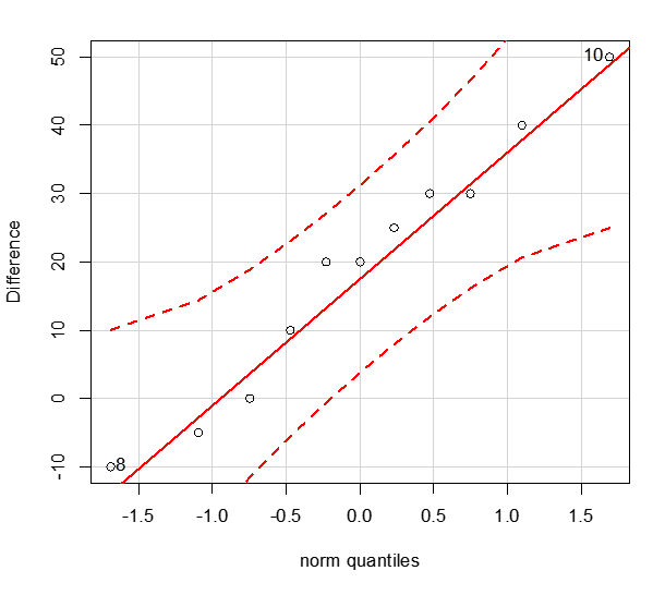
|
| 130 | 100 | 30 | 900 | |
| 140 | 115 | 25 | 625 | |
| 160 | 140 | 20 | 400 | |
| 110 | 115 | -5 | 25 | |
| 120 | 120 | 0 | 0 | |
| 150 | 130 | 20 | 400 | |
| 160 | 130 | 30 | 900 | |
| 100 | 110 | -10 | 100 | |
| 180 | 140 | 40 | 1600 | |
| 200 | 150 | 50 | 2500 | |
| 130 | 120 | 10 | 100 | |
| Sum | [latex]\sum d_i^2 =210[/latex] | [latex]\sum d_i^2 =7550[/latex] | ||
- Test at the 1% significance level whether the diet program is effective in reducing weight.
- Obtain a confidence interval corresponding to the test in part a).
- Does the interval in part b) support the conclusion in part a)?
- Is it possible to claim that the diet program can reduce weight by more than 5 pounds on average? Explain why.
Show/Hide Answer
Answer
- Check the assumptions:
- We have a simple random sample of paired differences.
- We have only n = 11 pairs, which is too small for the CLT to apply. Therefore, we should draw a Q-Q plot of the paired differences to see whether they are from a normal population. Since all the points are roughly on a straight line, there is no strong evidence against the normality assumption.
Let [latex]\mu_{\scriptsize B}[/latex] and [latex]\mu_{\scriptsize A}[/latex] be the mean weight before and after the diet program, respectively. If the diet program is effective in reducing weight, the average weight before the program should be larger than the average weight after the program.
Steps:
- Set up the hypotheses: [latex]H_0: \mu_{\scriptsize B} - \mu_{\scriptsize A} \leq 0[/latex] versus [latex]H_a: \mu_{\scriptsize B} - \mu_{\scriptsize A} \: \gt \: 0[/latex].
- The significance level is [latex]\alpha = 0.01[/latex].
- Compute the value of the test statistic:
[latex]t_o = \frac{\bar{d} - \delta_0}{s_d / \sqrt{n}} = \frac{19.091 - 0}{18.817 / \sqrt{11}} = 3.365[/latex] with [latex]df = n-1 = 11 - 1 = 10[/latex] and [latex]\bar{d} = \frac{\sum d_i}{n} = \frac{210}{11} = 19.091,[/latex] [latex]s_d = \sqrt{\frac{(\sum d_i^2) - \frac{(\sum d_i)^2}{n}}{n-1}} = \sqrt{ \frac{7550 - \frac{(210)^2}{11}}{11-1}} = 18.817[/latex]. - Find the P-value. For a right-tailed test, the P-value is the area to the right of the observed test statistic [latex]t_o[/latex], i.e.,
[latex]\mbox{P-value} = P(t \geq t_o) = P( t \geq 3.365) \Longrightarrow 0.0025<\text{P-value}<0.005.[/latex] Note that with [latex]df=10[/latex], [latex]3.169 (t_{0.005})<3.365<3.581 (t_{0.0025}).[/latex] - Decision: Since the P- value [latex]< 0.005 < 0.01(\alpha)[/latex], we reject the null hypothesis [latex]H_0[/latex].
- Conclusion: At the 1% significance level, the data provide sufficient evidence that the diet program is effective in reducing average weight.
- For a right-tailed test at the 1% significance level, the corresponding confidence interval is a 99% upper-tailed interval [latex](\bar{d} - t_{\alpha} \frac{s_d}{\sqrt{n}}, \infty)[/latex] with [latex]df = n-1 = 10,[/latex] [latex]t_{0.01} = 2.764, \bar{d} - t_{\alpha} \frac{s_d}{\sqrt{n}}= 19.091 - 2.764 \times \frac{18.817}{\sqrt{11}} = 3.409.[/latex] The 99% upper-tailed interval is [latex](3.409, \infty)[/latex].
Interpretation: We are 99% confident that the diet program reduces weight by at least 3.409 pounds on average. - Does the interval in part b) support the conclusion in part a)?
Yes. In part a), we reject [latex]H_0[/latex] and claim that [latex]\mu_{\scriptsize B} - \mu_{\scriptsize A} \: \gt \: 0[/latex]. In part b), since the interval does not contain [latex]\delta_0 = 0[/latex] and the entire interval is above 0, we are 99% confident that [latex]\mu_{\scriptsize B} - \mu_{\scriptsize A} \: \gt \: 0[/latex]. Thus, the results from part b) support the results obtained in part b). - Is it possible to claim that, on average, the diet program reduces weight by more than 5 pounds? Explain why.
This question asks us to test [latex]H_0: \mu_{\scriptsize B} - \mu_{\scriptsize A} \leq 5[/latex] versus [latex]H_a: \mu_{\scriptsize B} - \mu_{\scriptsize A} \: \gt \: 5[/latex]. Since the hypothesized difference [latex]\delta_0 = 5[/latex] is within the interval [latex](3.409, \infty)[/latex], we cannot reject 5 (or any value as low as 3.409) as a possible value for [latex]\mu_{\scriptsize A}[/latex] - [latex]\mu_{\scriptsize B}[/latex]. Therefore, we cannot reject [latex]H_0: \mu_{\scriptsize B} - \mu_{\scriptsize A} \leq 5[/latex].
