12.2 Main Idea Behind One-Way ANOVA
Let [latex]\mu_1, \mu_2, \dots , \mu_k[/latex] be [latex]k[/latex] population means. The hypotheses of one-way ANOVA are formulated as
[latex]H_0[/latex]: all means are equal, i.e., [latex]\mu_1 = \mu_2 = \dots = \mu_k[/latex]
[latex]H_a[/latex]: not all the means are equal.
The alternative hypothesis [latex]H_{a}[/latex] means there exists at least one pair of means that are not equal. Do not write as [latex]H_{a}: \mu_1 \neq \mu_2 \neq \dots \neq \mu_k[/latex]. Do not write “at least one mean is different from the others” since it sounds like at least one mean is different from the others while all the others are the same. Both are just two special cases of what "not all the means are equal" means.
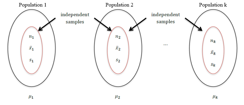
ANOVA F tests are based on [latex]k[/latex] independent, simple random samples from [latex]k[/latex] populations. If [latex]H_0: \mu_1 = \mu_2 = \dots = \mu_k[/latex] is true, the sample means [latex]\bar{x}_1, \bar{x}_2, \dots, \bar{x}_k[/latex] should be close to one another and hence, the variation among sample means should be small. Therefore, we should reject [latex]H_0[/latex] if the sample means are very different from one another (meaning the variation among the sample means would be large).
Quantifying Variation
The total variation of the data (SST: the total sum of squares) is quantified as the sum of squared distances from each observation to the overall mean, i.e., [latex]SST = \sum (x_{ij} - \bar{x})^2[/latex], where [latex]x_{ij}[/latex] is the [latex]j[/latex]th observation of sample [latex]i[/latex], [latex]\bar{x} = \frac{\sum x_{ij}}{n}[/latex] is the overall mean, and [latex]n = n_1 + n_2 + \dots + n_k[/latex] is the overall sample size.
The treatment sum of squares quantifies the variation of the sample means:
[latex]SSTR = \sum\limits_{i=1}^{k} n_i (\bar{x}_i - \bar{x})^2.[/latex]
SSTR quantifies the so-called between-group variation. For this reason, we should reject [latex]H_0: \mu_1 = \mu_2 = \dots = \mu_k[/latex] if SSTR is too large. However, SSTR is only considered "large" if it is large relative to the next measure of variation.
The within-group variation can be quantified as the sum of squared distances from each observation to the mean of its sample group, i.e.,
[latex]SSE = \sum (x_{ij} - \bar{x}_i)^2 = \sum_\limits{i=1}^k (n_i - 1) s_i^2.[/latex]
In practice, software is used to calculate all these sums of squares and other ANOVA calculations.
The total variation SST can be shown as:
[latex]SST = SSTR + SSE = \text{between group variation + within group variation}.[/latex]
The relationship between SSTR (between group variation) and SSE (within-group variation) will be illustrated in the following example.
A person recorded waiting times each time he called either Uber or Taxi service from his house and again each time he called either service from work. His results are summarized in the following table (red values correspond to waiting times for Uber and blue values correspond to Taxi):
Table 12.2: Waiting Time for Uber (red) and Taxi (blue) Called from Home and Work
| Home | 1 | 2 | 3 | 3 | 4 | 5 | 6 | 7 | 8 | 8 | 9 | 10 |
|---|---|---|---|---|---|---|---|---|---|---|---|---|
| Work | 1 | 2 | 3 | 3 | 4 | 5 | 6 | 7 | 8 | 8 | 9 | 10 |
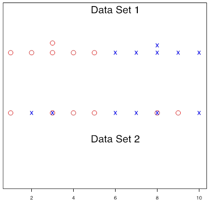
We define the waiting times called from Home as Data Set 1 and those called from Work as Data Set 2. The figure below shows two data sets. Each set consists of two populations: waiting time for Uber (red circle with mean [latex]\mu_1[/latex]) and waiting time for Taxi (blue cross with mean [latex]\mu_2[/latex]).

Exercise: Quantify Variation
Based on the two data sets shown above, answer these questions.
- The two data sets have (the same, different) total variation.
- Data set 1 has a (larger, smaller) within-group variation.
- Data set 1 has a (larger, smaller) between-group variation.
Support your answer by calculating the sums of squares [latex]SST, SSTR[/latex] and [latex]SSE[/latex] for each of the two groups.
Show/Hide Answer
Answers:
- The two data sets have the same total variation.
- Data set 1 has a smaller within-group variation.
- Data set 1 has a larger between-group variation.
The two data sets have the same overall sample mean [latex]\bar x[/latex] and the same total sum of square (SST):
[latex]\bar x=\frac{\sum x_i}{n}=\frac{1+2+3+3+4+5+6+7+8+8+9+10}{12}=5.5.[/latex]
[latex]\begin{align*}SST&=\sum (x_i-\bar x)^2\\&=(1-5.5)^2+(2-5.5)^2+(3-5.5)^2+\cdots+(8-5.5)^2+(9-5.5)^2\\&+(10-5.5)^2\\&=95.\end{align*}[/latex]
For Data Set 1, the mean waiting time for Uber is [latex]\bar x_1=\frac{1+2+3+3+4+5}{6}=3,[/latex] and the mean waiting time for Taxi is [latex]\bar x_2=\frac{6+7+8+8+9+10}{6}=8.[/latex] The between-group and within-group variation are:
[latex]SSTR=\sum n_i(\bar x_i-\bar x)=n_1(\bar x_1-\bar x)^2+ n_2(\bar x_2-\bar x)^2=6(3-5.5)^2+6(8-5.5)^2=75.[/latex]
[latex]\begin{align*}SSE&=\sum (x_{ij}-\bar x_i)^2\\&=(1-3)^2+(2-3)^2+(3-3)^2+(3-3)^2+(4-3)^2+(5-3)^2\\&+(6-8)^2+(7-8)^2+(8-8)^2+(8-8)^2+(9-8)^2+(10-8)^2\\&=10+10=20.\end{align*}[/latex]
For Data Set 2, the mean waiting time for Uber is [latex]\bar x_1=\frac{1+3+4+5+8+9}{6}=5,[/latex] and the mean waiting time for Taxi is [latex]\bar x_2=\frac{2+3+6+7+8+10}{6}=6.[/latex] The between-group and within-group variation are:
[latex]SSTR=\sum n_i(\bar x_i-\bar x)= n_1(\bar x_1-\bar x)^2+ n_2(\bar x_2-\bar x)^2=6(5-5.5)^2+6(6-5.5)^2=3.[/latex]
[latex]\begin{align*}SSE&=\sum (x_{ij}-\bar x_i)^2\\&=(1-5)^2+(3-5)^2+(4-5)^2+(5-5)^2+(8-5)^2+(9-5)^2\\&+(2-6)^2+(3-6)^2+(6-6)^2+(7-6)^2+(8-6)^2+(10-6)^2\\&=46+46=92.\end{align*}[/latex]
In both data sets, we have SST=SSTR+SSE. The two data sets have the same total variation SST=95. Data Set 1 has a smaller within-group variation SSE (20 versus 92). Data Set 1 has a larger between-group variation SSTR (75 versus 2).
For data set 1, it is clear that the data are from two populations with different means; for data set 2, however, it is hard to tell whether the data are from a single population or from two populations with similar means.
The main idea of one-way ANOVA is to decompose the total variation of the data (SST) into two parts: the variation within the samples (SSE) and the variation between sample means (SSTR). Reject [latex]H_0: \mu_1 = \mu_2 = \dots = \mu_k[/latex] if the variation between sample means is large compared to the variation within samples. Or reject [latex]H_0[/latex] if the ratio [latex]F = \frac{SSTR / (k-1)}{SSE / (n-k)} = \frac{MSTR}{MSE}[/latex] is too large, where MSTR is called the mean square of the treatments and MSE is the mean square error. The ratio follows an F distribution characterized by two degrees of freedom:
- The numerator degrees of freedom: [latex]df_n = k-1[/latex],
- The denominator degrees of freedom: [latex]df_d = n-k[/latex].
Like chi-square tests, F tests are always right-tailed. That is both the rejection region and the p-value are upper-tailed probabilities.
