11.4 Chi-Square Independence Test
The chi-square independence test is used to test for an association between two categorical variables of a population.
11.4.1 Terminologies Used for a Contingency Table
Recall that a contingency table summarizes the counts of two categorical variables. For example, the following contingency table groups 200 females according to their breast cancer status and smoking status:
Table 11.6: Contingency Table of Cancer Status (row) and Smoking Status (column)
|
Smoker [latex]\color{blue}{(S_1)}[/latex]
|
Non-smoker [latex]\color{blue}{(S_2)}[/latex]
|
Total | |
|---|---|---|---|
| Breast Cancer [latex]\color{red}{(C_1)}[/latex] | 10 [latex]( C_1 \: \& \: S_1 )[/latex] | 30 [latex]( C_1 \: \& \: S_2 )[/latex] | 40 |
| Cancer-free [latex]\color{red}{(C_2)}[/latex] | 20 [latex]( C_2 \: \& \: S_1 )[/latex] | 140 [latex]( C_2 \: \& \: S_2 )[/latex] | 160 |
| Total | 30 | 170 | 200 |
Suppose we randomly select an individual from this sample. Define the events:
[latex]\begin{align*} S_1 &= \text{the subject is a smoker}; \\ S_2 &= \text{the subject is a non-smoker}; \\ C_1 &= \text{the subject has breast cancer}; \\ C_2 &= \text{the subject does not have breast cancer.} \end{align*}[/latex]
The joint events are:
[latex]\begin{align*} C_1 \: \& \: S_1 &= \text{the subject has cancer and is a smoker}; \\ C_1 \: \& \: S_2 &= \text{the subject has cancer and is a non-smoker}; \\ C_2 \: \& \: S_1 &= \text{the subject does not have cancer and is a smoker}; \\ C_2 \: \& \: S_2 &= \text{the subject does not have cancer and is a non-smoker.} \end{align*}[/latex]
The variable “Cancer Status” is called the row variable, and it has two possible values—cancer or cancer-free. The variable “Smoking Status” is the column variable, and it has two values—smoker and non-smoker. The two numbers in the last column (40 and 160) are the row totals and the two in the last row (30, 170) are the column totals. The sample size is also called the grand total. The four numbers in bold are the joint frequencies. The boxes that contain the joint frequencies are referred to as cells.
Based on the [latex]\frac{f}{N}[/latex] rule, the marginal distribution of the row (column) variable equals the row (column) totals divided by [latex]n[/latex]. The joint distribution is given by the joint frequencies divided by [latex]n[/latex]. The following table shows the marginal distribution of “Cancer Status” in the last column, the marginal distribution of “Smoking Status” in the last row, and the joint distribution of the four cells.
Table 11.7: Marginal and Joint Probability Distributions of Cancer Status and Smoking Status
|
Smoker [latex]\color{blue}{(S_1)}[/latex]
|
Non-smoker [latex]\color{blue}{(S_2)}[/latex]
|
Total
|
|
|---|---|---|---|
|
Breast Cancer [latex]\color{red}{(C_1)}[/latex]
|
[latex]P(C_1 \: \& \: S_1) = \frac{10}{200} = 0.05[/latex] | [latex]P(C_1 \: \& \: S_2) = \frac{30}{200} = 0.15[/latex] | [latex]\color{red}{P(C_1) = \frac{40}{200} = 0.2}[/latex] |
|
Cancer-free [latex]\color{red}{(C_2)}[/latex]
|
[latex]P(C_2 \: \& \: S_1) =\frac{20}{200} = 0.1[/latex] | [latex]P(C_2 \: \& \: S_2) = \frac{140}{200} = 0.7[/latex] | [latex]\color{red}{P(C_1) = \frac{160}{200} = 0.8}[/latex] |
|
Total
|
[latex]\color{blue}{P(S_1) = \frac{30}{200} = 0.15}[/latex] | [latex]\color{blue}{P(S_2) = \frac{170}{200} = 0.85}[/latex] |
1
|
We want to test for an association between the two variables in a contingency table. Two variables are said to be associated if they are NOT independent. If two variables are associated, then differences exist among the conditional distributions of one variable, given different values of the other variable. For example, the conditional distributions of “Cancer Status” given “Smoking Status” are given in the following table. Notice that the conditional distributions are simply the relative frequencies of “Cancer” within smoker and non-smoker groups.
Table 11.8: Conditional Probability Distribution of Cancer Status Given Smoking Status
|
Smoker [latex]\color{blue}{(S_1)}[/latex]
|
Non-smoker [latex]\color{blue}{(S_2)}[/latex]
|
Marginal Distribution
Of Cancer Status |
|
|---|---|---|---|
|
Breast Cancer [latex]\color{red}{(C_1)}[/latex]
|
[latex]P(C_1 | S_1) = \frac{10}{30} = 0.333[/latex] | [latex]P(C_1 | S_2) = \frac{30}{170} = 0.176[/latex] | [latex]\color{red}{P(C_1) = \frac{40}{200} = 0.2}[/latex] |
|
Cancer-free [latex]\color{red}{(C_2)}[/latex]
|
[latex]P(C_2 | S_1) = \frac{20}{30} = 0.677[/latex] | [latex]P(C_2 | S_2) = \frac{140}{170} = 0.824[/latex] | [latex]\color{red}{P(C_2) = \frac{160}{200} = 0.8}[/latex] |
| Total |
1
|
1
|
1
|
A segmented bar graph helps us visualize conditional distributions and the concept of association. The figure below is the segmented bar graph that displays the conditional distributions of “Cancer Status” for smokers and non-smokers and the marginal distribution of "Cancer Status". The three bars should be identical if “Cancer Status” and “Smoking Status” are independent. That is, the conditional probabilities should equal the unconditional probabilities:
[latex]P(C_1 | S_1) = P(C_1 | S_2) = P(C_1); P(C_2 | S_1) = P(C_2 | S_2) = P(C_2).[/latex]
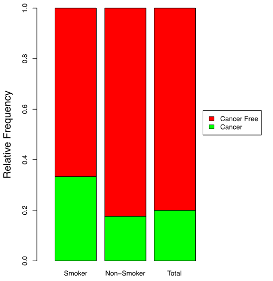 |
Interpretation:
The proportion or percentage of females with breast cancer (the green bar) is higher among the smokers than the non-smokers. Therefore, “Cancer Status” and “Smoking Status” might be associated; we can test this by a chi-square independence test. |
11.4.2 Main Idea Behind Chi-Square Independence Test
The null hypothesis is that the two variables are independent; the alternative is that they are associated. The test statistic is the same as that from the chi-square goodness-of-fit test; for each cell, compute the difference between the observed frequency (O) and the expected frequency ([latex]E[/latex]), square it, and divide by the expected frequency. The expected frequency is the number we expect to observe if the null is true. A large chi-square statistic means the observed and the expected frequencies are significantly different, which provides evidence against the null hypothesis. Therefore, we should reject the null if the observed chi-square statistic is sufficiently large. More specifically, given the significance level [latex]\alpha[/latex], reject [latex]H_0[/latex] if the P-value [latex]\leq \alpha[/latex], where the P-value is the area to the right of the observed test statistic under the chi-square curve.
The test procedure is straightforward—the key is calculating each cell's expected frequency. Recall that two events, A and B , are independent if [latex]P(A \: \& B) = P(A) \times P(B)[/latex]. For example, if the events “Breast Cancer” and “Smoker” are independent, then [latex]P(\text{Breast Cancer \& Smoker}) = P(\text{Breast Cancer}) \times P(\text{Smoker})[/latex] where [latex]P(\text{Breast Cancer})[/latex] and [latex]P(\text{Smoker})[/latex] are given by the marginal distribution of “Cancer Status” and “Smoking Status” respectively. That is,
[latex]P(\text{Breast Cancer}) = \frac{40}{200} = 0.2; P(\text{Smoker}) = \frac{30}{200} = 0.15.[/latex]
If [latex]H_0[/latex] (the two variables are independent) is true, the expected frequency for the cell “Cancer and Smoker” is
[latex]E = n P(\text{Cancer and Smoker}) = n P(\text{Cancer}) P(\text{Smoker})= 200 \times \frac{40}{200} \times \frac{30}{200} = \frac{40 \times 30}{200} = 6.[/latex]
In general,
[latex]\text{Expected frequency of the cell in rth row and cth column} = \frac{\text{rth row total} \times \text{cth column total}}{n}.[/latex]
Applying the above formula to each cell yields the following expected frequencies:
- "Cancer" & "Smoker": [latex]E = \frac{40 \times 30}{200} = 6.[/latex]
- "Cancer" & "Non-smoker": [latex]E = \frac{40 \times 170}{200} = 34.[/latex]
- "Cancer free" & "Smoker": [latex]E = \frac{160 \times 30}{200} = 24.[/latex]
- "Cancer free" & "Non-smoker": [latex]E = \frac{160 \times 170}{200} = 136.[/latex].
To compute the test statistic, it is helpful to write each expected frequency in the same cell as the corresponding observed frequency. The following table gives both the observed and expected frequencies for each cell (the expected frequencies are displayed in brackets):
Table 11.9: Observed and Expected Frequency (in Brackets) of Chi-Square Independent Test
|
Smoker [latex]\color{blue}{(S_1)}[/latex]
|
Non-smoker [latex]\color{blue}{(S_2)}[/latex]
|
Total | |
|---|---|---|---|
| Breast Cancer [latex]\color{red}{(C_1)}[/latex] | 10 (6) | 30 (34) | 40 |
| Cancer-free [latex]\color{red}{(C_2)}[/latex] | 20 (24) | 140 (136) | 160 |
| Total |
30
|
170
|
200 |
Chi-Square Independence Test
The assumptions and steps of conducting a chi-square independence test are as follows.
Assumptions:
- All expected frequencies are at least 1.
- At most 20% of the expected frequencies are less than 5.
- Simple random sample (required only if you need to generalize the conclusion to a larger population).
Note: If either assumption 1 or 2 is violated, one can consider combining the cells to make the counts in those cells larger.
Steps to perform a chi-square independence test:
First, check the assumptions. Calculate the expected frequency for each possible value of the variable using [latex]E = \frac{\text{rth row total} \times \text{cth column total}}{n}[/latex], where [latex]n[/latex] is the total number of observations. Check whether the expected frequencies satisfy assumptions 1 and 2. If not, consider combining some cells.
- Set up the hypotheses:
[latex]\begin{align*} H_0 &: \text{The two variables are independent} \\ H_a &: \text{The two variables are associated}. \end{align*}[/latex] - State the significance level [latex]\alpha[/latex].
- Compute the value of the test statistic: [latex]\chi_o^2 = \sum_{ \text{all cells}} \frac{(O- E)^2}{E}[/latex] with, [latex]df = (r-1) \times (c-1)[/latex] where [latex]E = \frac{\text{rth row total} \times \text{cth column total}}{n}[/latex], [latex]r[/latex] is the number of rows and [latex]c[/latex] is number of columns of the cells.
- Find the P-value or rejection region based on the [latex]\chi^2[/latex] curve with [latex]df = (r-1) \times (c-1)[/latex]
P-value [latex]P(\chi^2 \geq \chi_o^2)[/latex] the area to the right of [latex]\chi_o^2[/latex] under the curve Rejection region [latex]\chi^2 \geq \chi_{\alpha}^2[/latex] the region to the right of [latex]\chi_{\alpha}^2[/latex] - Reject the null [latex]H_0[/latex] if the P-value [latex]\leq \alpha[/latex] or [latex]\chi_o^2[/latex] falls in the rejection region.
- Conclusion.
Example: Chi-Square Independence Test
Test at the 10% significance level whether the variables “Cancer Status” and “Smoking Status” are associated.
|
Smoker (S1)
|
Non-smoker(S2)
|
Total | |
|---|---|---|---|
| Breast Cancer [latex]\color{red}{(C_1)}[/latex] | 10 (6) | 30 (34) | 40 |
| Cancer-free [latex]\color{red}{(C_2)}[/latex] | 20 (24) | 140 (136) | 160 |
| Total |
30
|
170
|
200 |
Check the assumptions: The expected frequencies are the values given in brackets, all greater than 5. We must assume this is a simple random sample of females.
Steps:
- Set up the hypotheses:
[latex]H_0: \text{The variables "Cancer Status" and "Smoking Status" are independent}[/latex]
[latex]H_a: \text{The variables "Cancer Status" and "Smoking Status" are associated.}[/latex] - The significance level is [latex]\alpha = 0.1[/latex].
- Compute the value of the test statistic:
[latex]\begin{align*}\chi_o^2 &= \sum_{\text{all cells}} \frac{(O-E)^2}{E}\\& = \frac{(10-6)^2}{6}+ \frac{(30-34)^2}{34}+ \frac{(20-24)^2}{24}+ \frac{(140-136)^2}{136} \\&= 3.922. \end{align*}[/latex]
with [latex]df = (r-1) \times (c-1) = (2-1) \times (2-1) = 1[/latex]. - Find the P-value:
[latex]\mbox{P-value}= P(\chi^2 \geq X_0^2) = P(\chi^2 \geq 3.992) \Longrightarrow 0.025 < \mbox{P-value} < 0.05[/latex] since [latex]3.841(\chi_{0.05}^2) < \chi_o^2=3.922 < 5.024 (\chi_{0.025}^2)[/latex]. - Decision: Reject the null [latex]H_0[/latex] sin,ce P-value [latex]\leq 0.05 < 0.1 (\alpha)[/latex].
- Conclusion: At the 10% significance level, we have sufficient evidence of an association between the variables “Cancer Status” and “Smoking Status”.

Exercise: Chi-Square Independence Test
A random sample of 230 adults yields the following data regarding age and Internet usage. At the 1% significance level, do the data provide sufficient evidence of an association between age and Internet usage?
Table 11.10: Contingency Table of Internet Usage (row) and Age (column)
|
18–24
|
25–64
|
65+
|
Total
|
|
|---|---|---|---|---|
|
Never
|
6
|
38
|
31
|
75
|
|
Sometimes
|
14
|
31
|
5
|
50
|
|
Every day
|
50
|
50
|
5
|
105
|
|
Total
|
70
|
119
|
41
|
230
|
Show/Hide Answer
Answers:
Check the assumptions.
Applying the formula [latex]\text{Expected frequency of the cell in rth row and cth column} = \frac{\text{rth row total} \times \text{cth column total}}{n}[/latex] to each cell, the expected frequencies are given by:
- "Never" & "18-24": [latex]E = \frac{75 \times 70}{230} = 22.826.[/latex]
- "Never" & "25-64": [latex]E = \frac{75 \times 119}{230} = 38.804.[/latex]
- "Never" & "65+": [latex]E = \frac{75 \times 41}{230} = 13.370.[/latex]
- "Sometimes" & "18-24": [latex]E = \frac{50 \times 70}{230} = 15.217.[/latex]
- "Sometimes" & "25-64": [latex]E = \frac{50 \times 119}{230} = 25.870.[/latex]
- "Sometimes" & "65+": [latex]E = \frac{50 \times 41}{230} = 8.913.[/latex]
- "Every day" & "18-24": [latex]E = \frac{105 \times 70}{230} = 31.957.[/latex]
- "Every day" & "25-64": [latex]E = \frac{105 \times 119}{230} = 54.326.[/latex]
- "Every day" & "65+": [latex]E = \frac{105 \times 41}{230} = 18.717.[/latex]
The expected frequencies are given in brackets; they are all greater than 5. We are told this is a random sample. Therefore, assumptions for the chi-square independence test are satisfied.
Table 11.11: Observed and Expected Frequency of Internet Usage (row) and Age (column)
|
18–24
|
25–64
|
65+
|
Total
|
|
|---|---|---|---|---|
|
Never
|
6 (22.826)
|
38 (38.804)
|
31 (13.370)
|
75
|
|
Sometimes
|
14 (15.217)
|
31 (25.870)
|
5 (8.913)
|
50
|
|
Every day
|
50 (31.957)
|
50 (54.326)
|
5 (18.717)
|
105
|
|
Total
|
70
|
119
|
41
|
230
|
Steps:
- Set up the hypotheses:
[latex]\begin{align*} H_0 &: \text{The variables "Age" and "Internet usage" are independent} \\ H_a &: \text{The variables "Age" and "Internet usage" are associated}. \end{align*}[/latex] - The significance level is [latex]\alpha = 0.01[/latex].
- Compute the value of the test statistic:
[latex]\begin{align*}\chi_o^2 &= \sum_{\text{all cells}} \frac{(O-E)^2}{E} \\&= \frac{(6-22.826)^2}{22.826}+ \frac{(38-38.804)^2}{38.804}+ \frac{(31-13.370)^2}{13.370} +\frac{(14-15.217)^2}{15.217}\\&+ \frac{(31-25.870)^2}{25.870}+ \frac{(5-8.913)^2}{8.913}+ \frac{(50-31.957)^2}{31.957} +\frac{(50-54.326)^2}{54.326}\\&+\frac{(5 - 18.717)^2}{18.717}= 59.084. \end{align*}[/latex]
with
[latex]df = (r-1) \times (c-1) = (3-1) \times (3-1) = 4[/latex].
- Find the P-value: P-value= [latex]P(\chi^2 \geq \chi_o^2) = P(\chi^2 \geq 59.084) < 0.005[/latex].
- Decision: Reject the null [latex]H_0[/latex] since P-value [latex]\leq 0.005 < 0.01 (\alpha)[/latex].
- Conclusion: At the 1% significance level, we have sufficient evidence that there is an association between age and Internet usage.
