12.4 One-Way ANOVA F Test
The assumptions and steps of a one-way ANOVA F test are as follows.
Assumptions:
- Normal populations: the variable of interest is normally distributed for each population.
- Equal variances: the variance of the variable of interest is the same for all populations.
- Independent samples: the samples from different populations are independent of one another.
- Simple random samples: the samples taken from the [latex]k[/latex] populations are simple random samples.
Steps:
- Set up the hypotheses:
[latex]\begin{align*} H_0 &: \mu_1 = \mu_2 = \dots = \mu_k\\ H_a&: \text{Not all means are equal.}\end{align*}[/latex] - State the significance level [latex]\alpha[/latex].
- Calculate the sums of squares SST, SSTR, SSE and the mean squares MSTR, MSE. Find the test statistic, [latex]F_o[/latex], and show the results in an ANOVA table:
Source [latex]df[/latex][latex]SS[/latex][latex]MS = \frac{SS}{df}[/latex]F-statisticp-valueTreatment [latex]k-1[/latex][latex]SSTR[/latex][latex]MSTR = \frac{SSTR}{k-1}[/latex][latex]F_o = \frac{MSTR}{MSE}[/latex][latex]P(F \geq F_o)[/latex]Error [latex]n-k[/latex][latex]SSE[/latex][latex]MSE = \frac{SSE}{n-k}[/latex]Total [latex]n-1[/latex][latex]SST[/latex] - Find the P-value or rejection region based on the F density curve with degrees of freedom [latex]df_n = k-1, df_d = n-k[/latex].
P-value [latex]P(F \geq F_o)[/latex] the area to the right of [latex]F_o[/latex] under the curve Rejection region [latex]F \geq F_{\alpha}[/latex] the region to the right of the critical value [latex]F_{\alpha}[/latex] - Reject the null [latex]H_0[/latex] if P-value [latex]\leq \alpha[/latex] or [latex]F_o[/latex] falls in the rejection region.
- Conclusion.
Example: One-Way ANOVA F Test on Download Time
The following ANOVA table corresponds to the download time example. Use the information in this ANOVA table to test at the 1% significance level whether there is a significant difference between the mean download times at 7 a.m., 5 p.m., and 12 a.m.
Table 12.4: ANOVA Table of Download Time Example
| Source |
[latex]df[/latex]
|
[latex]SS[/latex]
|
[latex]MS = \frac{SS}{df}[/latex]
|
F-statistic
|
P-value
|
|---|---|---|---|---|---|
| Time of day |
[latex]2[/latex]
|
[latex]204641[/latex]
|
[latex]102320[/latex]
|
[latex]F_o = 46.03[/latex]
|
[latex]< 0.0001[/latex]
|
| Error |
[latex]45[/latex]
|
[latex]100020[/latex]
|
[latex]2223[/latex]
|
||
| Total |
[latex]47[/latex]
|
[latex]304661[/latex]
|
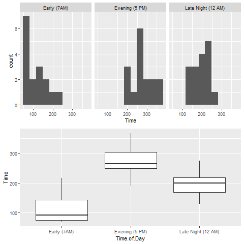
The side-by-side histograms and boxplots of all three groups can be found below. Both the side-by-side histograms and boxplots show that the downloading time at 7 AM, 5 PM and 12 AM is not normally distributed, since the histograms are not bell-shaped and the boxplots are not symmetric. The side-by-side boxplots show that the median downloading time of 7 AM, 5 PM, and 12 AM are around 90, 260, and 200 minutes respectively.
Steps to conduct a one-way ANOVA F test:
- Hypotheses
[latex]H_0: \mu_1 = \mu_2 = \mu_3[/latex]
[latex]H_a: \text{Not all means are equal}[/latex]. - The significance level is [latex]\alpha = 0.01[/latex].
- The test statistic is [latex]F_o = 46.03[/latex] with [latex]df_n = k-1 = 3-1 =2, df_d = n-k = 48 -3 =45[/latex].
- P-value [latex]P(F \geq F_o) = P(F \geq 46.03) < 0.0001[/latex] (given in the ANOVA table)
- Reject [latex]H_0[/latex], since p-value [latex]< 0.0001 < 0.01 (\alpha)[/latex].
- Conclusion: At the 1% significance level, we have sufficient evidence that there is a significant difference among the mean download times at 7 a.m., 5 p.m., and 12 a.m.

Exercises: One-Way ANOVA F Test
Many studies have suggested that there is an association between exercise and healthy bones. One study examined the effect of jumping on the bone density of growing rats. There are three treatments: a control with no jumping, a low-jump condition (the jump height was 30 centimetres), and a high-jump condition (60 centimetres). After eight weeks of 10 jumps per day, five days per week, the bone density of the rats in milligrams per cubic centimetre (mg/cm3) was measured. The data are given in the following table.
Table 12.5: Bone Density for Three Treatments
| Group | Bone density | Group | Bone density | Group | Bone density |
| Control | 611 | Low jump | 635 | High jump | 650 |
| Control | 621 | Low jump | 605 | High jump | 622 |
| Control | 614 | Low jump | 638 | High jump | 626 |
| Control | 593 | Low jump | 594 | High jump | 626 |
| Control | 593 | Low jump | 699 | High jump | 631 |
| Control | 653 | Low jump | 632 | High jump | 622 |
| Control | 600 | Low jump | 631 | High jump | 643 |
| Control | 554 | Low jump | 588 | High jump | 674 |
| Control | 603 | Low jump | 607 | High jump | 643 |
| Control | 569 | Low jump | 596 | High jump | 650 |
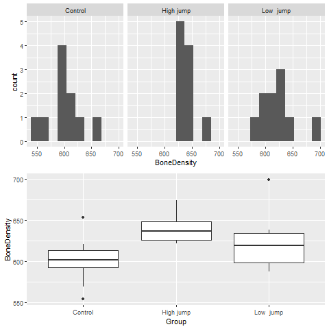
The side-by-side histograms and boxplots are shown as follows:
Given the ANOVA table, test at the 5% significance level whether jumping strengthens the bones of rats.
Table 12.6: ANOVA Table of Bone Density Exercise
| Source |
[latex]df[/latex]
|
[latex]SS[/latex]
|
[latex]MS = \frac{SS}{df}[/latex]
|
F-statistic
|
P-value
|
|---|---|---|---|---|---|
| Group |
[latex]2[/latex]
|
[latex]7114[/latex]
|
[latex]3557[/latex]
|
[latex]F_o = 5.08[/latex]
|
[latex]0.0133[/latex]
|
| Error |
[latex]27[/latex]
|
[latex]18879[/latex]
|
[latex]699[/latex]
|
||
| Total |
[latex]29[/latex]
|
[latex]25993[/latex]
|
Show/Hide Answer
Answers:
Steps to conduct a one-way ANOVA F test:
- Hypotheses
[latex]H_0: \mu_1 = \mu_2 = \mu_3[/latex]
[latex]H_a: \text{Not all means are equal}[/latex]. - The significance level is [latex]\alpha = 0.05[/latex].
- The test statistic is [latex]F_o = 5.08[/latex] with [latex]df_n = k-1 = 3-1 = 2, df_d = n-k = 30-3 = 27[/latex].
- P-value [latex]= P(F \geq F_o) = P(F \geq 5.08) < 0.0133[/latex] (given in the ANOVA table)
- Reject [latex]H_0[/latex], since p–value [latex]= 0.0133 < 0.05 (\alpha)[/latex].
- Conclusion: At the 5% significance level, we have sufficient evidence that the mean bone densities are different in the three treatment groups. Since the rats in the "high jump" group has the largest mean bone density, followed by the "low jump" group, we can conclude that jumping strengthens the bones of rats.
