8.2 Type I and Type II Errors
In testing hypotheses, there are only two possible outcomes: either reject [latex]H_0[/latex] or do not reject [latex]H_0[/latex]; in reality, there are only two possible scenarios: either [latex]H_0[/latex] is true or [latex]H_0[/latex] is false. Hence, regardless of which conclusion we make, we have a chance to make an error. There are two types of errors: Type I and Type II.
Type I error: reject the null [latex]H_0[/latex] when [latex]H_0[/latex] is in fact true.
Type II error: do not reject the null [latex]H_0[/latex] when [latex]H_0[/latex] is false.
Table 8.2: Type I and Type II Error
|
[latex]H_0[/latex] is True
|
[latex]H_0[/latex] is False
|
|
|---|---|---|
| Decision: Do not reject [latex]H_0[/latex] | Correct decision | Type II error |
| Decision: Reject [latex]H_0[/latex] | Type I error | Correct decision |
The probability of type I error is denoted as [latex]\alpha[/latex], and the probability of type II error is denoted as [latex]\beta[/latex]. That is:
[latex]\alpha = P(\text{Type I error}) = P(\text{Reject }H_0|H_0 \text{ is true})[/latex]
[latex]\beta = P(\text{Type II error}) = P(\text{Do not reject }H_0|H_0 \text{ is false})[/latex]
The type I error rate [latex]\alpha[/latex] is also called the significance level of a hypothesis test.
Example: Type I and Type II Errors
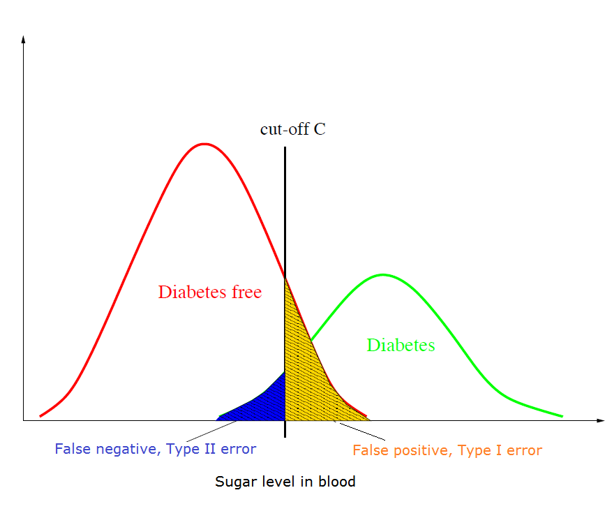
In a diabetes blood test, a patient is diagnosed with the disease if the sugar level in their bloodstream is larger than the threshold C=130 mg/dL. Suppose the distributions of sugar levels for the two populations (diabetes-free and having diabetes) are the two bell-shaped curves shown in the following figure.
Define the hypotheses: [latex]H_0[/latex] (a patient is disease free) vs. [latex]H_a[/latex] (a patient has diabetes). What are the type I and type II errors in this example?
Type I error: claim the person has diabetes (reject the null [latex]H_0[/latex]) but actually the person does not have diabetes ([latex]H_0[/latex] is in fact true). This is often referred to as a false positive.Type II error: claim the person does not have diabetes(do not reject the null [latex]H_0[/latex]), but actually the person has diabetes ([latex]H_0[/latex] is false). This is often referred to as a false negative.
The figure in the above example shows the trade-off between type I and type II errors. The gold area gives [latex]\alpha[/latex], the probability of the type I error; and the blue area gives [latex]\beta[/latex], the probability of the type II error. If we increase the threshold C (move the cut-off to the right), the gold area will reduce and the blue area will increase. That is the type I error rate [latex]\alpha[/latex] will decrease and the type II error rate [latex]\beta[/latex] will increase. On the other hand, if we reduce the threshold C (move the cut-off to the left), the type I error rate [latex]\alpha[/latex] will increase and the type II error rate will decrease. This is the trade-off between the type I and type II errors [latex]\alpha[/latex] and [latex]\beta[/latex]. It is not a good idea to set either [latex]\alpha[/latex] or [latex]\beta[/latex] to be too close to 0; otherwise, the other error rate will be huge. For example, if we set the threshold C very large, few individuals will be diagnosed as diabetic; as a result, many diabetic individuals will be misclassified as not having the disease (meaning we have a high probability of committing a type I error). On the other hand, if we set the threshold C very small, most individuals will be diagnosed as diabetic; consequently, many individuals who are free of diabetes will be misclassified as diabetic (meaning we have a high probability of committing a type II error). In general, we can set [latex]\alpha[/latex] (or [latex]\beta[/latex]) to be relatively small if the consequence of the type I (or type II) error is more serious. The power of a test is defined as
[latex]1 - \beta = 1- P(\text{Type II error})[/latex] [latex]= 1 - P(\text{Do not reject } H_0 | H_0 \text{ false}) = P(\text{Reject } H_0 | H_0 \text{ false}).[/latex]
This is the probability that we reject [latex]H_0[/latex] when [latex]H_0[/latex] is false. Thus, it is of interest for a statistical test to have a high level of power.

Exercise: Type I and Type II Errors
Suppose you are performing a statistical test to decide whether a nuclear reactor should be approved. The null hypothesis is that the reactor is safe to use, and so failing to reject the null hypothesis corresponds to approval.
- Write down the null and alternative hypotheses.
- What are the type I and type II errors in this example?
- Which error has a more serious consequence, type I or type II? Which of [latex]\alpha[/latex] or [latex]\beta[/latex] should be smaller?
Show/Hide Answer
Answers:
- [latex]H_0[/latex]: the nuclear reactor is safe versus [latex]H_a[/latex]: the nuclear reactor is not safe.
- Type I error: disapprove the nuclear reactor for use given that the nuclear reactor is actually safe.
Type II error: approve the nuclear reactor for use given that the nuclear reactor is not safe. - The type II error is more serious than the type I. Disapproving a safe reactor would waste time and money, but approving an unsafe reactor could lead to a nuclear meltdown, which is a catastrophic event. For this reason, we should set the type II error rate [latex]\beta[/latex] to be relatively small.
