6.3 Central Limit Theorem (CLT)
The central limit theorem is one of the most important theorems in statistics.
Key Fact: The Central Limit Theorem
When a random sample of size n is drawn from any population with mean [latex]\mu[/latex] and standard deviation [latex]\sigma[/latex] , the distribution of the sample mean [latex]\bar{X}[/latex] will be (approximately) normally distributed if the sample size n is large enough. In general, [latex]n \geq 30[/latex] is large enough if the population distribution is not too extremely skewed.
Note that:
- The central limit theorem is about the shape of the distribution of the sample mean [latex]\bar{X}[/latex]. It is the distribution of the random variable [latex]\bar{X}[/latex] that will be normally distributed if the sample size n is large enough.
- The required sample size n depends on how skewed the population distribution is. If the population distribution, the distribution of [latex]X[/latex], is symmetric, [latex]n \geq 5[/latex] might be large enough to claim that the sample mean [latex]\bar{X}[/latex] is approximately normally distributed; if the distribution of [latex]X[/latex] is not too extremely skewed, [latex]n \geq 30[/latex] should be enough; if the population is very skewed, we might need [latex]n \geq 100[/latex] (see the central limit theorem for proportion in Chapter 10).
In addition to the results on the mean and standard deviation of [latex]\bar{X}[/latex], we can claim that:
Key Fact: The Distribution of the Sample Mean [latex]\color{white} \bar{X}[/latex]
For a normal population or large sample, the sample mean [latex]\bar{X}[/latex] follows a normal distribution with mean [latex]\mu_{\scriptsize \bar{X}} = \mu[/latex] and standard deviation [latex]\sigma_{\scriptsize \bar{X}} = \frac{\sigma}{\sqrt{n}}[/latex]. That is [latex]\bar{X} \sim N(\mu, \frac{\sigma}{\sqrt{n}})[/latex].
Example: Distribution of the sample mean [latex]\color{white} \bar{X}[/latex]
- Let [latex]X[/latex] denote student grades in a particular class, and suppose [latex]X[/latex] is normally distributed with a mean of 70 and a standard deviation of 10, i.e., [latex]X \sim N(\mu=70, \sigma = 10)[/latex].
- If I randomly pick four students, determine the distribution of their average grade. Indicate the mean, standard deviation, and shape.
Mean: [latex]\mu_{\scriptsize \bar{X}} = \mu = 70[/latex].
Standard deviation: [latex]\sigma_{\scriptsize \bar{X}} = \frac{\sigma}{\sqrt{n}} = \frac{10}{\sqrt{4}} = 5[/latex].
Shape: normal since the population is normal. Recall that when the population distribution is normal, the distribution of the sample mean [latex]\bar{X}[/latex] is also normal regardless of the sample size.
Therefore, the average grade of four randomly selected students [latex]\bar{X} \sim N(\mu_{\scriptsize \bar{X}}=70, \sigma_{\scriptsize \bar{X}} = 5)[/latex]. - If I randomly pick 100 students, determine the distribution of their average grade. Indicate the mean, standard deviation, and shape.
Mean: [latex]\mu_{\scriptsize \bar{X}} = \mu = 70[/latex].
Standard deviation: [latex]\sigma_{\scriptsize \bar{X}} = \frac{\sigma}{\sqrt{n}} = \frac{10}{\sqrt{100}} = 1[/latex].
Shape: normal since the population is normal. Recall that when the population distribution is normal, the distribution of the sample mean [latex]\bar{X}[/latex] is also normal regardless of the sample size.
Therefore, the average grade of 100 randomly selected students [latex]\bar{X} \sim N(\mu_{\scriptsize \bar{X}}=70, \sigma_{\scriptsize \bar{X}} = 1)[/latex]. - If I randomly pick four students, find the probability that their average is between 60 and 90.
By part (a), for [latex]n = 4[/latex], average grade [latex]\bar{X} \sim N(\mu_{\scriptsize \bar{X}} = 70, \sigma_{\scriptsize \bar{X}} = 5)[/latex] . Therefore,
[latex]\begin{align*}P(60 \leq \bar{X} \leq 90)&= P \left( \frac{60 - \mu_{\scriptsize \bar{X}}}{\sigma_{\scriptsize \bar{X}}} \leq \frac{\bar{X} - \mu_{\scriptsize \bar{X}}}{\sigma_{\scriptsize \bar{X}}} \leq \frac{90 - \mu_{\scriptsize \bar{X}}}{\sigma_{\scriptsize \bar{X}}} \right)\\ &= P \left( \frac{60 - 70}{5} \leq Z \leq \frac{90 - 70}{5} \right)\\ &=P(-2 \leq Z \leq 4)\\ &= P( Z \leq 4) - P(Z \leq -2) \\ &= 1 - 0.0228 = 0.9772. \end{align*}[/latex]
- If I randomly pick four students, determine the distribution of their average grade. Indicate the mean, standard deviation, and shape.
- Suppose the lifetime of a brand of laptops follows an extremely right-skewed distribution with a mean [latex]\mu = 5[/latex] years and a standard deviation [latex]\sigma = 5[/latex].
- If I randomly pick four laptops, determine the distribution of their average lifetime. Indicate the mean, standard deviation, and shape.
Mean: [latex]\mu_{\scriptsize \bar{X}} = \mu = 5[/latex] years.
Standard deviation: [latex]\sigma_{\scriptsize \bar{X}} = \frac{\sigma}{\sqrt{n}} = \frac{5}{\sqrt{4}} = 2.5[/latex] years.
Shape: Not normal, still right-skewed. The population is extremely right-skewed, and the sample size [latex]n=4[/latex] is too small to apply the central limit theorem. - If I randomly pick 100 laptops, determine the distribution of their average lifetime. Indicate the mean, standard deviation, and shape.
Mean: [latex]\mu_{\scriptsize \bar{X}} = \mu = 5[/latex] years.
Standard deviation: [latex]\sigma_{\scriptsize \bar{X}} = \frac{\sigma}{\sqrt{n}} = \frac{5}{\sqrt{100}} = 0.5[/latex] years.
Shape: approximately normal. The population is extremely right-skewed, but the sample size [latex]n = 100 \: > \: 30[/latex] is large enough to apply the central limit theorem. Therefore, [latex]\bar{X} \sim N(\mu_{\scriptsize \bar{X}}=5, \sigma_{\scriptsize \bar{X}} = 0.5)[/latex]. - If I randomly pick 100 laptops, find the probability that their average lifetime is at least four years.
By part (b), for [latex]n=100[/latex], the average lifetime [latex]\bar{X} \sim N(\mu_{\scriptsize \bar{X}}=5, \sigma_{\scriptsize \bar{X}} = 0.5)[/latex]. Hence,
[latex]\begin{align*}P(\bar{X} \geq 4)&= P \left( \frac{\bar{X} - \mu_{\scriptsize \bar{X}}}{\sigma_{\scriptsize \bar{X}}} \geq \frac{4 - \mu_{\scriptsize \bar{X}}}{\sigma_{\scriptsize \bar{X}}} \right)\\ &= P \left( Z \geq \frac{4 - 5}{0.5} \right)= P(Z \geq -2) \\ &=P(Z \leq 2) = 0.9722. \end{align*}[/latex]
- If I randomly pick four laptops, determine the distribution of their average lifetime. Indicate the mean, standard deviation, and shape.
Exercise: Distribution of the Sample Mean
Let [latex]X=[/latex] the rent of a one-bedroom apartment in Edmonton, and suppose that [latex]X[/latex] follows a distribution with a mean of $700 and a standard deviation of $400. The distribution of [latex]X[/latex] (the population distribution) is given by the density curve below.
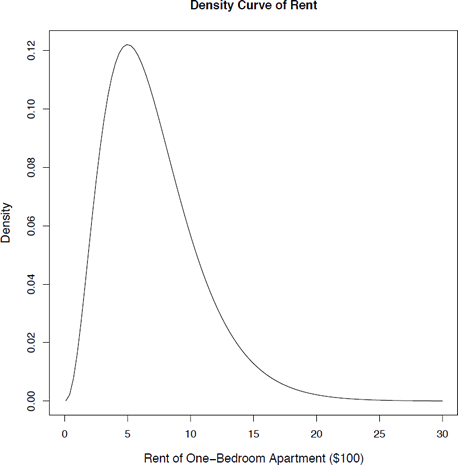
- Describe the population distribution of the rent of a one-bedroom apartment in Edmonton, i.e., the distribution of [latex]X[/latex]. Comment on modality, center, spread, and shape.
- If you randomly pick four one-bedroom apartments, describe the sampling distribution of their average rent. Indicate the mean, standard deviation, and shape.
- If you randomly pick 100 one-bedroom apartments, describe the sampling distribution of their average rent. Indicate the mean, standard deviation, and shape.
- If you randomly pick 100 one-bedroom apartments, find the probability that their average rent is above $800.
Show/Hide Answer
- Unimodal, right skewed, centered at the mean 700 with a spread of 400 as the standard deviation.
- Mean: [latex]\mu_{\scriptsize \bar{X}} = \mu = $700[/latex].
Standard deviation: [latex]\sigma_{\scriptsize \bar{X}} = \frac{\sigma}{\sqrt{n}} = \frac{400}{\sqrt{4}} = $200[/latex].
Shape: Not normal, still right-skewed. The population is right-skewed, and the sample size [latex]n=4[/latex] is too small to apply the central limit theorem.
- Mean: [latex]\mu_{\scriptsize \bar{X}} = \mu = $700[/latex].
Standard deviation: [latex]\sigma_{\scriptsize \bar{X}} = \frac{\sigma}{\sqrt{n}} = \frac{400}{\sqrt{100}} = $40[/latex].
Shape: approximately normal. The population is right-skewed, but the sample size [latex]n = 100 \: > \: 30[/latex], so it is large enough to apply the central limit theorem.
- By part (c), [latex]n = 100[/latex] for, the average rent [latex]\bar{X} \sim N(\mu_{\scriptsize \bar{X}}=700, \sigma_{\scriptsize \bar{X}}=40)[/latex]. Hence,
[latex]\begin{align*} P(\bar{X} \geq 800) &= P \left( \frac{\bar{X} - \mu_{\scriptsize \bar{X}}}{\sigma_{\scriptsize \bar{X}}} \geq \frac{800 - \mu_{\scriptsize \bar{X}}}{\sigma_{\scriptsize \bar{X}}} \right) \\ &= P \left( Z \geq \frac{800-700}{40} \right) \\ &= P(Z \geq 2.5) \\ &= P(Z \leq -2.5) \\ &=0.0062. \end{align*}[/latex]
