6.5 Review Questions
- Explain the relationship between the population mean [latex]\mu[/latex], sample mean [latex]\bar X[/latex], and a value of the sample mean [latex]\bar x[/latex]. Which is the population parameter, which is an estimate and which is an estimator?
- [latex]P(Z<-4)[/latex] = ________; [latex]P(Z<5)[/latex] = ________; [latex]P(Z>5)[/latex] = ________.
- Which of the following statements about the distribution of the sample mean are true?
- The distribution of the sample mean is never exactly normal.
- The sample mean will be approximately normally distributed when the population is large enough.
- When the sample size is at least 30, the sample mean is always approximately normally distributed. (just a rule of thumb, when the population is NOT extremely skewed))
- When the sample size is large enough, the sample mean will be approximately normally distributed.
- When the population distribution is normal, the sample mean will be exactly normally distributed regardless of the sample size.
- When the sample size is small, the sample mean will never be normally distributed.
- When the sample size is large enough, the population distribution will be approximately normally distributed.
- Is the following statement about the central limit theorem correct? If it is not correct, could you modify it to make it correct? “When the sample size is greater than 30, it follows a normal distribution".
- Suppose random variable [latex]X[/latex] is normally distributed with mean 40 and standard deviation 4. Consider all possible random samples of size [latex]n = 4[/latex] from this population, and find the mean, standard deviation, and shape of the sample mean [latex]\bar X[/latex].
- The time that a technician requires to perform preventive maintenance on an air-conditioning unit is known to have an extremely right-skewed distribution with a mean of 1.2 hours and a standard deviation of 1.2 hours. Consider all possible random samples of size [latex]n = 4[/latex] from this population, and find the mean, standard deviation, and shape of the sample mean [latex]\bar X[/latex].
- Suppose that [latex]X[/latex], the rent of a one-bedroom apartment in Edmonton, follows a distribution with a mean of $800 and a standard deviation of $400. Its density curve is given below.
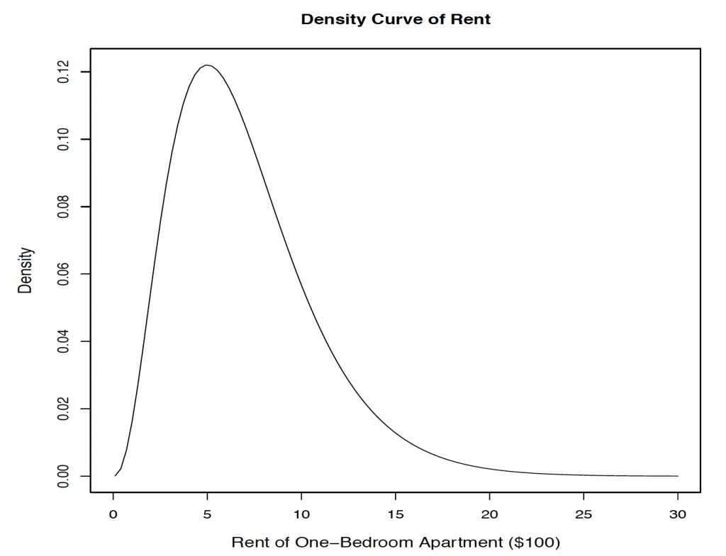
[Image Description (See Appendix D Chapter 6 Question 7)] - If you randomly pick four one-bedroom apartments, describe the sampling distribution of their average rent. Indicate the mean, standard deviation, and shape.
- If you randomly pick 64 one-bedroom apartments, describe the sampling distribution of their average rent. Indicate the mean, standard deviation, and shape.
- If randomly pick 64 one-bedroom apartments, find the probability that their average rent is below $980.
- Fill in the following table about the mean, the standard deviation, and the shape of [latex]X[/latex] (the variable of interest, the population) and sample mean [latex]\bar X[/latex] with different sample size [latex]n[/latex].
Variable Mean Standard Deviation Shape [latex]X[/latex] (population) [latex]\mu =[/latex] [latex]\sigma =[/latex] Not normal, right skewed [latex]\bar X[/latex] (sample mean) with [latex]n = 4[/latex] [latex]\mu_{\scriptsize \bar X} =[/latex] [latex]\sigma_{\scriptsize \bar X} =[/latex] [latex]\bar X[/latex] with [latex]n = 64[/latex] [latex]\mu_{\scriptsize \bar X} =[/latex] [latex]\sigma_{\scriptsize \bar X} =[/latex]
Show/Hide Answer
- The population mean [latex]\mu[/latex] is used to describe the population, [latex]\mu[/latex] is a constant but in general unknown. The sample mean [latex]\bar{X}[/latex] is a random variable, and it is an estimator of [latex]\mu[/latex]; its value depends on the sample; the sample mean [latex]\bar{x}[/latex] is a possible value of [latex]\bar{X}[/latex] based on one sample, [latex]\bar{x}[/latex] is also a point estimate of [latex]\mu[/latex].
- [latex]P(Z < - 4) = 0[/latex]; [latex]P(Z < 5) = 1[/latex]; [latex]P(Z > 5) = 0[/latex].
- False
If the population distribution is normal, the distribution of the sample mean [latex]\bar{X}[/latex] is always exactly normal regardless of the sample size [latex]n[/latex]. - False
When the sample size n is large enough, the sample mean [latex]\bar{X}[/latex] will be approximately normally distributed. - False
Sample size [latex]n \geq 30[/latex] is just a rule of thumb. It is true only when the population is NOT extremely skewed. - True, CLT
- True
- False
If the population distribution is normal, the distribution of the sample mean [latex]\bar{X}[/latex] is always exactly normal regardless of the sample size [latex]n[/latex]. - False
The CLT is about the shape of the distribution of the sample mean [latex]\bar{X}[/latex]; it has nothing to do with the population distribution.
- False
- The problem of this statement is what “it” refers to. We can modify it to “When the sample size is large enough, the sample mean [latex]X[/latex] is approximately normal.”
- The mean of the sample mean equals the population mean: [latex]\mu_{\scriptsize \bar{X}} = \mu = 40[/latex].
The standard deviation of the sample mean equals the population standard deviation divided by the square root of the sample size [latex]n[/latex]: [latex]\sigma_{\bar{X}} = \frac{\sigma}{n} = \frac{4}{\sqrt{4}} = 2.[/latex]
The shape of the sample mean [latex]\bar{X}[/latex] is normal, exactly normal, since the population is normal. - The mean of the sample mean equals the population mean: [latex]\mu_{\scriptsize \bar{X}} = \mu = 1.2[/latex] hours.
The standard deviation of the sample mean equals the population standard deviation divided by the square root of the sample size [latex]n[/latex]: [latex]\sigma_{\bar{X}} = \frac{\sigma}{n} = \frac{1.2}{\sqrt{4}} = 0.6.[/latex]
The shape of the sample mean [latex]\bar{X}[/latex] is not normal, still right skewed, because the population is right skewed and the sample size [latex]n = 4[/latex] is too small to apply the central limit theorem. - This question is almost identical to the Exercise: Distribution of the Sample Mean in Section 6.3.
- Mean: [latex]\mu_{\scriptsize \bar{X}} = \mu = $800[/latex].
Standard deviation: [latex]\sigma_{\scriptsize \bar{X}} = \frac{\sigma}{\sqrt{n}} = \frac{400}{\sqrt{4}} = $200[/latex].
Shape: Not normal, still right-skewed. The population is right-skewed, and the sample size [latex]n=4[/latex] is too small to apply the central limit theorem. - Mean: [latex]\mu_{\bar{X}} = \mu = $800[/latex].
Standard deviation: [latex]\sigma_{\scriptsize \bar{X}} = \frac{\sigma}{\sqrt{n}} = \frac{400}{\sqrt{64}} = $50[/latex].
Shape: approximately normal. The population is right-skewed, but the sample size [latex]n = 64 \: > \: 30[/latex], so it is large enough to apply the central limit theorem. - By part (b), [latex]n = 64[/latex] for, the average rent [latex]\bar{X} \sim N(\mu_{\bar{X}}=800, \sigma_{\bar{X}}=50)[/latex]. Hence,[latex]\begin{align*} P(\bar{X} < 980) &= P \left( \frac{\bar{X} - \mu_{\scriptsize \bar{X}}}{\sigma_{\scriptsize \bar{X}}} < \frac{980 - \mu_{\scriptsize \bar{X}}}{\sigma_{\scriptsize \bar{X}}} \right) \\ &= P \left( Z \geq \frac{980-800}{50} \right) \\ &= P(Z < 3.6) \\ &= 0.9998. \end{align*}[/latex]
- The filled-in table is as follows.
- Mean: [latex]\mu_{\scriptsize \bar{X}} = \mu = $800[/latex].
| Variable | Mean | Standard Deviation | Shape |
|---|---|---|---|
| [latex]X[/latex] (population) | [latex]\mu = 800[/latex] | [latex]\sigma = 400[/latex] | Not normal, right skewed |
| [latex]\bar X[/latex] (sample mean) with [latex]n = 4[/latex] | [latex]\mu_{\scriptsize \bar X} = 800[/latex] | [latex]\sigma_{\scriptsize \bar X} = \frac{400}{\sqrt{4}}=200[/latex] | Not normal right skewed |
| [latex]\bar X[/latex] with [latex]n = 100[/latex] | [latex]\mu_{\scriptsize \bar X} = 800[/latex] | [latex]\sigma_{\scriptsize \bar X} = \frac{400}{\sqrt{64}}=50[/latex] | Approximately normal |
