1.8 Assignment 1
Purposes
This assignment has two parts. The first part assesses your knowledge of the concept of sample, population, descriptive vs. inferential study, using graphs to summarize data. The second part assesses your skills in using R commander to create the graphs and interpreting their meaning.
Resources
Instructions
Part A
Important note:
By default, in all assignments in this course, you are required to complete the questions or tasks in Part A by hand. This means that to do any calculation or drawing, you will NOT use R commander or any computer application. That is, you will do calculations manually with a non-programmable scientific calculator and use a pen or pencil to draw figures or build a distribution table on paper (or drawing pad/tablet) and take a photo of it and insert it below the answer space of the question. Before you start your assignment, you should get a calculator that has Statistic functions.
Before you complete Part B using R commander, you should read and practice the R commander steps by following the guidance in the Lab Manual.
Complete the following:
- In order to investigate the effectiveness of a new method in teaching STAT 151 at MacEwan University. From all students who are taking or who will be taking STAT 151 at MacEwan University, a simple random sample of 800 students were selected for this study. From these 800 students, a simple random sample of 200 students were chosen and assigned to sections taught with the new method, while the other 600 were taught with the standard method. At the end of the term, the class average in the final grade for students taught with the new method is 3% higher than that for students taught with the regular method.
- Identify the sample and population of this study. (2 marks)
- Is this study a designed experiment or an observational study? Explain why. (2 marks)
- Is this study descriptive or inferential? Explain why. (2 marks)
- Propose two different methods to take a simple random sample of 200 students from a collection of 800 students. (2 marks)
- The following table shows the prices of 30 sale homes (in the last column) and 9 features of the homes: size (area of the home measured in square feet), pool (indicating whether the property has a swimming pool or not), area (total area of the lot in square feet), age (age of the home), bath (# of bathrooms), stories (# of stories), garage (# of cars can be parked), traffic (whether the property faces street subject to a constant flow of daily traffic), roof (whether the home has a tile roof or non-tile roof).
Note: the following data is the first 30 ones on the spreadsheet of M01_SaleHome.xlsx you will download for the Part B tasks.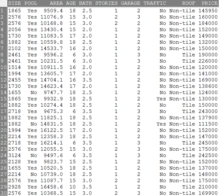
[Image Description (See Appendix D Question 2)] - Identify the type of data provided in each column as qualitative, quantitative discrete, or quantitative continuous. (10 marks)
- For the variable “size,” (total 10 marks)
- Obtain a frequency distribution using [1400, 1600) as the first sub-interval, [1600, 1800) as the second sub-interval, [1800, 2000) as the third, and etc. and insert it in the space below. (2 marks)
- Obtain a relative frequency distribution based on part (1) and insert it in the space below. (2 marks)
- Construct a relative-frequency histogram and insert it below. (3 marks)
- Describe the graph you constructed in part (3) about its overall shape, modality, symmetricity/skewness, if applicable. (3 marks)
- For the variable “bath,” do the following: (total 9 marks)
- Obtain a frequency distribution. (2 marks)
- Obtain a relative frequency distribution based on part (1). (2 marks)
- Construct a graph corresponding to part (1). (3 marks)
- Describe the graph obtained in part (3). (2 marks)
- For the variable “roof,” do the following: (total 12 marks)
- Obtain a frequency distribution. (2 marks)
- Obtain a relative frequency distribution based on part (1). (2 marks)
- Construct two different types of graphs corresponding to part (2). (6 marks)
- Describe the graphs obtained in part (3). (2 marks)
Part B
Finish the following questions using R and R commander:
Read the data set “M01_SaleHome.xlsx” and use R commander to complete the following tasks. For each, you need to copy or do a screenshot of the output in R commander (we later call it computer output) and paste it into the space below the questions. To save space, you only need to copy and paste what is asked for in the questions, and sometime may need to shrink the size.
- Use the most suitable type of graphs to summarize the prices of these 88 sale homes. Comment on the distribution of the price in terms of overall shape, modality, symmetricity/skewness if applicable. (5 marks)
- Use a suitable graph(s) we taught in Module 1 to compare the prices of homes with a tile roof and a non-tile roof. Briefly explain your findings based on the graph(s). (5 marks)
- Use R commander to obtain a contingency table with “roof” as the row variable and “pool” as the column variable (2 marks).
Based on the computer outputs from R commander, obtain the percentages in the following four questions.- Homes with a swimming pool. (1 mark)
- Homes without a swimming pool. (1 mark)
- Homes with a swimming pool and with a tile roof. (1 mark)
- Homes without a swimming pool and with a non-tile roof. (1 mark)
- Use the most suitable graph to show the effect of “Size” on the “Price” of the sale home. Briefly describe the relationship you found. (5 marks)
