5.1 Density Curve
We use a density curve to describe the distribution of a continuous variable. A density curve is the continuous analogue of a relative-frequency histogram with the density (scaled relative frequency) as the y-axis. For example, 1,000 grades are shown in the following grouping table and the relative-frequency histogram. The total area of the bins in the relative-frequency histogram is
[latex]\text{area} = 10 \times 0.003 + 10 \times 0.019 + 10 \times 0.150 + \cdots+ 10 \times 0.144 + 10 \times 0.022 = 10.[/latex]
The total area of the three leftmost bins is
[latex]\text{area}= 10 \times 0.003 + 10 \times 0.019 + 10 \times 0.150 = 1.72[/latex],
which accounts for [latex]1.72/10=0.172[/latex] or [latex]1.72\%[/latex] of the data. If we re-scale the y-axis of the relative-frequency histogram by dividing relative frequency (probability) by 10 (the bin width) and draw a smooth curve on the top of the histogram, we obtain the density curve of the grades with the y-axis density = relative frequency/width of the bins = relative frequency/10.
|
 |
 |
||||||||||||||||||
| Table 5.1: Grouping Table of Grade | Figure 5.1: Probability Histogram (Left) and Density Curve (Right) of Grade. [Image Description (See Appendix D Figure 5.1)] Click on image to enlarge. | |||||||||||||||||||
Let [latex]X=[/latex] grade, the proportion of grades below 60 is given by
[latex]\begin{align*} P(X < 60) &= 0.003 + 0.019 + 0.150 = 0.172\\ &= \text{total area of the leftmost three bins}\\ &= \text{area to the left of 60 under the red curve}. \end{align*}[/latex]
Similarly, the percentage of grades above 80, [latex]P(X \: > \: 80) = 0.144 + 0.022 -= 0.166[/latex], which is the total area of the rightmost two bins or the area to the right of 80 under the red curve. The proportion (percentage) of grades between 60 and 80 is given by
[latex]\begin{align*} P(60 < X < 80) &= 0.330 + 0.332 = 0.662\\ &= \text{total are of the two bins in the middle}\\ &= \text{the area between 60 and 80 under the red curve}. \end{align*}[/latex]
A density curve has the following properties:
Key Facts: Properties of a density curve
- Total area under the curve is one.
- Area of a region under the curve gives the probability of an event.
 |
 |
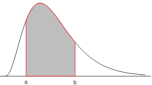 |
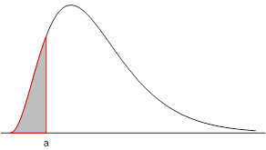
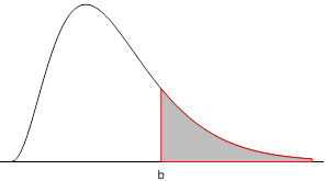
|
[latex]P(X \leq a)[/latex] probability below a = area to the left of a |
[latex]P(X \geq b)[/latex] probability above b = area to the right of b |
[latex]P(a \leq X \leq b)[/latex] [latex]= P(X \leq b) - P(X \leq a)[/latex] probability between a and b = area between a and b = area left of b minus area left of a. |
