9.2 Two-Sample t Test and t Interval Based on Two Independent Samples
Two-sample t-tests are used to test hypotheses regarding the difference between two population means. Depending on whether the two population standard deviations ([latex]\sigma_1[/latex] and [latex]\sigma_2[/latex]) are equal or not, we have the non-pooled and pooled two-sample t-tests and t interval. Minor advantages of the pooled t-test are a slightly narrower confidence interval, a slightly more powerful test, and a simpler formula for the degrees of freedom. However, the pooled t-test is valid only when the two population standard deviations are close; otherwise, it gives poor results. Therefore, we recommend using the non-pooled t-test unless we are quite confident that [latex]\sigma_1[/latex] = [latex]\sigma_2[/latex], which is very difficult to verify.
9.2.1 Non-Pooled Two-Sample t Test and t Interval
Assumptions:
- Simple random samples
- Two samples are independent
- Normal populations or large sample sizes [latex](n_1 \geq 30, n_2 \geq 30)[/latex]
Steps:
- Set up the hypotheses:
Two-tailed test
Right (upper)-tailed test
Left (lower)-tailed test
[latex]H_0: \mu_1 - \mu_2 = \Delta_0[/latex][latex]H_0: \mu_1 - \mu_2 \leq \Delta_0[/latex][latex]H_0: \mu_1 - \mu_2 \geq \Delta_0[/latex][latex]H_a: \mu_1 - \mu_2 \neq \Delta_0[/latex][latex]H_a: \mu_1 - \mu_2 \: \gt \: \Delta_0[/latex][latex]H_a: \mu_1 - \mu_2 \: \lt \: \Delta_0[/latex]Note that [latex]\Delta_0[/latex] can be zero or any value you want to test. In most cases, however, [latex]\Delta_0=0[/latex].
- State the significance level [latex]\alpha[/latex].
- Compute the value of the test statistic: [latex]t_o = \frac{(\bar{x}_1 - \bar{x}_2) - (\Delta_0)}{\sqrt{ \frac{s_1^2}{n_1} + \frac{s_2^2}{n_2}}}[/latex] with [latex]df = \frac{ \left( \frac{s_1^2}{n_1} + \frac{s_2^2}{n_2} \right)^2}{\frac{1}{n_1 - 1} \left( \frac{s_1^2}{n_1} \right)^2 + \frac{1}{n_2 - 1} \left( \frac{s_2^2}{n_2} \right)^2 }[/latex], rounded down to the nearest integer or [latex]\min\{n_1 -1, n_2 - 1 \}[/latex].
- Use the t-score table (Table IV) to find the P-value or rejection region.
Two-tailedRight-tailedLeft-tailed
Null [latex]H_0: \mu_1 - \mu_2 = \Delta_0[/latex][latex]H_0: \mu_1 - \mu_2 \leq \Delta_0[/latex][latex]H_0: \mu_1 - \mu_2 \geq \Delta_0[/latex]Alternative [latex]H_a: \mu_1 - \mu_2 \neq \Delta_0[/latex][latex]H_a: \mu_1 - \mu_2 \: \gt \: \Delta_0[/latex][latex]H_a: \mu_1 - \mu_2 \: \lt \: \Delta_0[/latex]P-value [latex]2P(t \geq |t_o|)[/latex][latex]P(t \geq t_o)[/latex][latex]P(t \leq t_o)[/latex]Rejection region [latex]t \geq t_{\alpha / 2}[/latex] or [latex]t \leq - t_{\alpha / 2}[/latex] [latex]t \geq t_{\alpha}[/latex][latex]t \leq - t_{\alpha}[/latex] - Decision: Reject the null [latex]H_0[/latex] if P-value [latex]\leq \alpha[/latex] or [latex]t_o[/latex] falls in the rejection region.
- Conclusion.
A [latex](1 –\alpha) \times 100\%[/latex] two-sample [latex]t[/latex] confidence interval for [latex]\mu_1[/latex] – [latex]\mu_2[/latex] is
|
Two-tailed
|
Right-tailed
|
Left-tailed
|
|---|---|---|
|
[latex]H_0: \mu_1 - \mu_2 = \Delta_0[/latex]
|
[latex]H_0: \mu_1 - \mu_2 \leq \Delta_0[/latex]
|
[latex]H_0: \mu_1 - \mu_2 \geq \Delta_0[/latex]
|
|
[latex]H_a: \mu_1 - \mu_2 \neq \Delta_0[/latex]
|
[latex]H_a: \mu_1 - \mu_2 \: \gt \: \Delta_0[/latex]
|
[latex]H_a: \mu_1 - \mu_2 \: \lt \: \Delta_0[/latex]
|
| [latex](\bar{x}_1 - \bar{x}_2) \pm t_{\alpha / 2} \sqrt{ \frac{s_1^2}{n_1} + \frac{s_2^2}{n_2}}[/latex] | [latex]\left((\bar{x}_1 - \bar{x}_2) - t_{\alpha} \sqrt{ \frac{s_1^2}{n_1} + \frac{s_2^2}{n_2}}, \infty \right)[/latex] | [latex]\left(- \infty , (\bar{x}_1 - \bar{x}_2) + t_{\alpha} \sqrt{ \frac{s_1^2}{n_1} + \frac{s_2^2}{n_2}}\right)[/latex] |
Example: Two-Sample Non-Pooled t-Test and t Interval
Some students attend class regularly, but some do not. An instructor wants to compare the class averages for those who attend lectures regularly ([latex]\mu_1[/latex]) with those who do not ([latex]\mu_2[/latex]). A simple random sample of size [latex]n_1 = 135[/latex] is selected from the attendees and a simple random sample of size [latex]n_2=35[/latex] is taken from the non-attendees. The sample mean and sample standard deviation for attendees are [latex]\bar{x}_1 = 67, s_1 = 17[/latex]; and for non-attendees are [latex]\bar{x}_2 = 49, s_2 = 18[/latex].
- Test at the 1% significance level whether those who attend lectures have a higher average, i.e., [latex]\mu_1 \: \gt \: \mu_2[/latex] or [latex]\mu_1 - \mu_2 \: \gt \: 0[/latex].
Check the assumptions:
- We have simple random samples from attendees and non-attendees.
- The two samples are independent.
- We do not have the data, so we cannot check whether two populations are normally distributed using normal probability plot (Q-Q plot); however, we have large sample sizes with [latex]n_1 = 135 \: \gt \: 30, n_2 = 35 \: \gt \: 30[/latex].
Therefore, the assumptions are met.
Steps:
- Set up the hypotheses: [latex]H_0: \mu_1 - \mu_2 \leq 0[/latex] versus [latex]H_a: \mu_1 - \mu_2 \: \gt \: 0[/latex].
This is a right-tailed test. - The significance level is [latex]\alpha=0.01[/latex].
- Compute the value of the test statistic:
[latex]t_o = \frac{(\bar{x}_1 - \bar{x}_2) - \Delta_0}{\sqrt{ \frac{s_1^2}{n_1} + \frac{s_2^2}{n_2}}} = \frac{(67 - 49) -0}{\sqrt{ \frac{17^2}{135} + \frac{18^2}{35}}} = 5.332[/latex] with
[latex]df = \frac{ \left( \frac{s_1^2}{n_1} + \frac{s_2^2}{n_2} \right)^2}{\frac{1}{n_1 - 1} \left( \frac{s_1^2}{n_1} \right)^2 + \frac{1}{n_2 - 1} \left( \frac{s_2^2}{n_2} \right)^2 } = \frac{ \left( \frac{17^2}{135} + \frac{18^2}{35} \right)^2}{\frac{1}{135 - 1} \left( \frac{17^2}{135} \right)^2 + \frac{1}{35 - 1} \left( \frac{18^2}{35} \right)^2 } = 50.85[/latex], rounded down to [latex]df = 50[/latex].
- Find the P-value. For a right-tailed test with the observed test statistics [latex]t_o=5.332[/latex], the P-value is the area to the right of [latex]t_o[/latex], i.e., [latex]\mbox{P-value} = P(t \geq t_o) = P(t \geq 5.332) < 0.0005, \mbox{since} t_o=5.332 \: \gt \: 3.496(t_{0.0005})[/latex]
- Decision: Since the P-value [latex]< 0.0005 < 0.01 (\alpha)[/latex], reject the null hypothesis [latex]H_0[/latex].
- Conclusion: At the 1% significance level, the data provide sufficient evidence that those who attend lectures have a higher average.
If using the critical value approach, steps 1-3 are the same, steps 4-6 become:
-
- Rejection region:
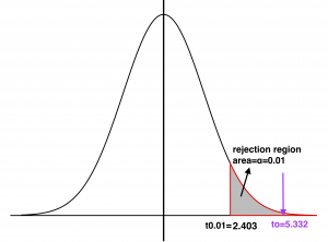
Figure 9.2: Rejection Region and Observed Value. [Image Description (See Appendix D Figure 9.2)] [latex]\alpha = 0.01 , t_{\alpha} = t_{0.01} = 2.403[/latex] For a right-tailed test, the critical value is 2.403. The rejection region is to the right of 2.403.
- Decision: Since the observed value [latex]t_o =5.332 \: \gt \: 2.403[/latex] falls in the rejection region, we reject the null hypothesis [latex]H_0[/latex].
- Conclusion: At the 1% significance level, the data provide sufficient evidence that those who attend lectures have a higher average.
- Rejection region:
- Obtain a confidence interval for the difference between the class average for attendees and non-attendees [latex]\mu_1 - \mu_2[/latex] corresponding to the test in part a).
Part a) contains a right-tailed test at the 1% significance level. Therefore, we should obtain a 99% upper-tailed interval: [latex]\left((\bar{x}_1 - \bar{x}_2) - t_{\alpha} \sqrt{ \frac{s_1^2}{n_1} + \frac{s_2^2}{n_2}}, \infty \right)[/latex].
[latex]\alpha = 0.01, df = 50, t_{\alpha} = t_{0.01} = 2.403[/latex].
The lower bound for the upper-tailed interval is:[latex](\bar{x}_1 - \bar{x}_2) - t_{\alpha} \sqrt{ \frac{s_1^2}{n_1} + \frac{s_2^2}{n_2}} = (67 - 49) - 2.403 \times \sqrt{ \frac{17^2}{135} + \frac{18^2}{35}} = 9.887[/latex].
Thus, the corresponding 99% confidence interval for [latex]\mu_1 - \mu_2[/latex] is [latex](9.887, \infty)[/latex].
Interpretation: we are 99% confident that the difference in average grades is at least 9.887 between attendees and non-attendees. - Does the interval in part (b) support the conclusion in part a)?
In part a), we reject [latex]H_0[/latex] at the 1% significance level and claim that [latex]\mu_1 - \mu_2 \: \gt \: 0[/latex].
In part b), since the entire interval is above 0, we can claim that [latex]\mu_1 - \mu_2 \: \gt \: 0[/latex] with 99% confidence, which supports the results obtained in part a). - Based on the interval obtained in part b), can we claim that the class average of attendees is at least 5 marks higher than that of the non-attendees? How about 10 marks higher?
We can claim that the class average of attendees is at least 5 marks higher than that of the non-attendees since the entire interval is above 5. However, we cannot claim that the class average of attendees is at least 10 marks higher than that of the non-attendees since the interval contains 10.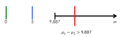
Figure 9.3: Confidence Interval of difference in Class Average. [Image Description (See Appendix D Figure 9.3)]
9.2.2 Pooled Two-Sample t Test and t Interval
If the two population standard deviations are equal, i.e., [latex]\sigma_1 = \sigma_2 = \sigma[/latex], we can pool the two samples together to get a better estimate of the common standard deviation [latex]\sigma[/latex]
[latex]\hat{\sigma} = s_p = \sqrt{ \frac{(n_1 - 1)s_1^2 + (n_2 -1)s_2^2 } {(n_1 - 1) + (n_2 -1)}}[/latex]
where the term [latex](n_1 - 1)s_1^2 = \sum_{\text{sample 1}}(x - \bar{x}_1)^2[/latex] is the variation of the data within sample 1, and [latex](n_2 - 1)s_2^2 = \sum_{\text{sample 2}}(x - \bar{x}_2)^2[/latex] is the variation of the data within sample 2.
Recall that the standard deviation of [latex]\bar{X}_1 - \bar{X}_2[/latex] is [latex]\sigma_{\scriptsize \bar{X}_1 - \bar{X}_2} = \sqrt{ \frac{\sigma_1^2}{n_1} + \frac{\sigma_2^2}{n_2} }[/latex]. Thus, if [latex]\sigma_1 = \sigma_2 = \sigma[/latex], then [latex]\sigma_{\scriptsize \bar{X}_1 - \bar{X}_2}[/latex] reduces to [latex]\sqrt{ \frac{\sigma^2}{n_1} + \frac{\sigma^2}{n_2} } = \sigma \sqrt{ \frac{1}{n_1} + \frac{1}{n_2} }[/latex]. Estimating [latex]\sigma[/latex] with [latex]s_p[/latex] leads to the pooled test statistic:
[latex]t = \frac{(\bar{X}_1 - \bar{X}_2) - (\mu_1 - \mu_2)}{s_p \sqrt{\frac{1}{n_1} + \frac{1}{n_2} } } \sim \text{$t$ distribution}[/latex]
with [latex]df = (n_1 - 1) + (n_2 -1) = n_1 + n_2 -2[/latex].
The assumption [latex]\sigma_1 = \sigma_2[/latex] is very difficult to verify. Some textbooks suggest a rule of thumb:
If the ratio of the larger to the smaller sample standard deviation is less than 2, then the assumption is considered to be reasonable, i.e., [latex]\frac{\max \{ s_1, s_2\}}{\min \{ s_1, s_2\}} < 2[/latex].
Assumptions:
- Simple random samples.
- Independent samples.
- Normal populations or large sample sizes [latex](n_1 \geq 30, n_2 \geq 30)[/latex].
- Equal population standard deviations. This assumption is reasonable if [latex]\frac{\max \{ s_1, s_2\}}{\min \{ s_1, s_2\}} < 2[/latex].
Steps:
- Set up the hypotheses:
Two-tailed test Right (upper)-tailed test Left (lower)-tailed test [latex]H_0: \mu_1 - \mu_2 = \Delta_0[/latex][latex]H_0: \mu_1 - \mu_2 \leq \Delta_0[/latex][latex]H_0: \mu_1 - \mu_2 \geq \Delta_0[/latex][latex]H_a: \mu_1 - \mu_2 \neq \Delta_0[/latex][latex]H_a: \mu_1 - \mu_2 \: \gt \: \Delta_0[/latex][latex]H_a: \mu_1 - \mu_2 \: \lt \: \Delta_0[/latex]Note that [latex]\Delta_0[/latex] can be zero or any value you want to test.
- State the significance level [latex]\alpha[/latex].
- Compute the value of the test statistic: [latex]t_o = \frac{(\bar{x}_1 - \bar{x}_2) - \Delta_0}{s_p \sqrt{ \frac{1}{n_1} + \frac{1}{n_2}}}[/latex], with [latex]df = n_1 + n_2 – 2[/latex] and [latex]s_p = \sqrt{ \frac{(n_1 - 1)s_1^2 + (n_2 -1)s_2^2 } {(n_1 - 1) + (n_2 -1)}}[/latex].
- Use the t-score table (Table IV) to find the P-value or rejection region.
Two-tailedRight-tailedLeft-tailedNull [latex]H_0: \mu_1 - \mu_2 = \Delta_0[/latex][latex]H_0: \mu_1 - \mu_2 \leq \Delta_0[/latex][latex]H_0: \mu_1 - \mu_2 \geq \Delta_0[/latex]Alternative [latex]H_a: \mu_1 - \mu_2 \neq \Delta_0[/latex][latex]H_a: \mu_1 - \mu_2 \: \gt \: \Delta_0[/latex][latex]H_a: \mu_1 - \mu_2 \: \lt \: \Delta_0[/latex]P-value [latex]2P(t \geq |t_o|)[/latex][latex]P(t \geq t_o)[/latex][latex]P(t \leq t_o)[/latex]Rejection region [latex]t \geq t_{\alpha / 2}[/latex] or [latex]t \leq - t_{\alpha / 2}[/latex] [latex]t \geq t_{\alpha}[/latex][latex]t \leq - t_{\alpha}[/latex] - Decision: Reject the null [latex]H_0[/latex] if P-value [latex]\leq \alpha[/latex] or [latex]t_o[/latex] falls in the rejection region.
- Conclusion.
A [latex](1 - \alpha) \times 100%[/latex] two-sample t confidence interval for [latex]\mu_1 - \mu_2[/latex] is
|
Two-tailed
|
Right-tailed
|
Left-tailed
|
|---|---|---|
|
[latex]H_0: \mu_1 - \mu_2 = \Delta_0[/latex]
|
[latex]H_0: \mu_1 - \mu_2 \leq \Delta_0[/latex]
|
[latex]H_0: \mu_1 - \mu_2 \geq \Delta_0[/latex]
|
|
[latex]H_a: \mu_1 - \mu_2 \neq \Delta_0[/latex]
|
[latex]H_a: \mu_1 - \mu_2 \: \gt \: \Delta_0[/latex]
|
[latex]H_a: \mu_1 - \mu_2 \: \lt \: \Delta_0[/latex]
|
| [latex]\small{(\bar{x}_1 - \bar{x}_2) \pm t_{\alpha / 2} s_p \sqrt{ \frac{1}{n_1} + \frac{1}{n_2}}}[/latex] | [latex]\small{\left((\bar{x}_1 - \bar{x}_2) - t_{\alpha} s_p \sqrt{ \frac{1}{n_1} + \frac{1}{n_2}}, \infty \right)}[/latex] | [latex]\small{\left(- \infty , (\bar{x}_1 - \bar{x}_2) + t_{\alpha} s_p \sqrt{ \frac{1}{n_1} + \frac{1}{n_2}}\right)}[/latex] |
Example: Pooled Two-Sample t Test and Interval
Some students attend class regularly, but some do not. An instructor wants to compare the class averages for those who attend lectures regularly ([latex]\mu_1[/latex]) with those who do not ([latex]\mu_2[/latex]). A simple random sample of size [latex]n_1=135[/latex] is selected from the attendees, and a simple random sample of size [latex]n_2=35[/latex] is taken from the non-attendees. The sample mean and sample standard deviation for attendees are [latex]\bar{x}_1 = 67, s_1 = 17[/latex]; and for non-attendees are [latex]\bar{x}_2 = 49, s_2 = 18[/latex].
- Is it reasonable to conduct a pooled two-sample t-test to test whether those who attend lectures have a higher average? If yes, run the test at the 1% significance level.
Check the assumptions:
- We have simple random samples.
- The two samples are independent.
- We have large sample sizes [latex](n_1 = 135 > 30, n_2 =35 > 30)[/latex].
- Equal standard deviation [latex]\frac{\max \{ s_1, s_2 \} }{\min \{ s_1, s_2 \}} = \frac{\max \{ 17, 18 \}}{\min \{ 17, 18 \}} = \frac{18}{17} < 2[/latex].
It is reasonable to conduct a pooled two-sample t-test since all the assumptions for pooled two-sample t-test are met.
Steps:
-
- Set up the hypotheses: [latex]H_0: \mu_1 - \mu_2 \leq 0[/latex] versus [latex]H_a: \mu_1 - \mu_2 \: \gt \: 0[/latex]. This is a right-tailed test.
- The significance level is [latex]\alpha=0.01[/latex].
- Compute the value of the test statistic:
[latex]t_o = \frac{(\bar{x}_1 - \bar{x}_2) - \Delta_0}{s_p \sqrt{ \frac{1}{n_1} + \frac{1}{n_2}}} = \frac{(67-49) - 0}{17.207 \sqrt{ \frac{1}{135} + \frac{1}{35}}} = 5.515[/latex] with [latex]df = n_1 + n_2 – 2 = 135+35–2=168[/latex] (not given in Table IV, use df=100), and with
[latex]s_p = \sqrt{ \frac{(n_1 - 1)s_1^2 + (n_2 -1)s_2^2 } {n_1 + n_2 -2}} = \sqrt{ \frac{(135 - 1)17^2 + (35 -1)18^2 } {135 + 35 - 2}} = 17.207.[/latex] - Find the P-value. For a right-tailed test with the observed test statistics [latex]t_o=5.515[/latex], the P-value is the area to the right of [latex]t_o[/latex] i.e., p-value [latex]=P(t \geq t_o) = P(t \geq 5.515) < 0.0005[/latex], since [latex]t_o=5.515 \: \gt \: 3.390 (t_{0.0005})[/latex] with [latex]df=100[/latex].
- Decision: Since the P-value [latex]<0.0005< 0.01(\alpha)[/latex] reject the null hypothesis [latex]H_0[/latex]
- Conclusion: At the 1% significance level, the data provide sufficient evidence that those who attend lectures have a higher average.
- Obtain a confidence interval for the difference between the class average for attendees and non-attendees, [latex]\mu_1 - \mu_2[/latex], corresponding to the test in part a).
Part a) contains a right-tailed test at the 1% significance level. Therefore, we should obtain a 99% upper-tailed interval [latex]((\bar{x}_1 - \bar{x}_2) - t_{\alpha} s_p \sqrt{\frac{1}{n_1} + \frac{1}{n_2} }, \infty)[/latex], with [latex]\alpha=0.01, df=100[/latex], and [latex]t_{0.01}=2.364[/latex]. The lower bound for the upper-tailed interval is [latex]\begin{align*} (\bar{x}_1 - \bar{x}_2) - t_{\alpha} s_p \sqrt{\frac{1}{n_1} + \frac{1}{n_2} } &= (67 - 49) - 2.364 \times 17.207 \times \sqrt{\frac{1}{135} + \frac{1}{35}} \\ &= 10.284. \end{align*}[/latex] Thus, the corresponding 99% confidence interval for [latex]\mu_1 - \mu_2[/latex] is [latex](10.284, \infty)[/latex].
Interpretation: we are 99% confident that the difference in average grades is at least 10.284 between attendees and non-attendees. - Based on the confidence interval in part b), can we claim that the class average of attendees is at least 10 marks higher than that of the non-attendees?
Yes, since the entire interval is above 10, we can claim that [latex]\mu_1 - \mu_2 \: \gt \: 10[/latex].

Exercise: Two-Sample Test
The following table summarizes the operative times of neurosurgeries conducted by a dynamic system (Z-plate) and a static system (ALPS plate).
Table 9.1: Operating Time of Dynamic and Static System
|
Dynamic
|
Static
|
|
[latex]\bar{x}_1 = 400[/latex]
|
[latex]\bar{x}_2 = 480[/latex]
|
|
[latex]s_1 = 85[/latex]
|
[latex]s_2 = 40[/latex]
|
|
[latex]n_1 = 60[/latex]
|
[latex]n_2 = 30[/latex]
|
- Test at the 5% significance level whether the dynamic system (Z-plate) has a lower mean operative time than the static system (ALPS plate).
- Obtain a confidence interval for the difference in mean operative time between the dynamic and the static systems, [latex]\mu_1 - \mu_2[/latex], corresponding to the test in part a).
Show/Hide Answer
- Check the assumptions:
- We have simple random samples.
- The two samples are independent.
- We have large sample sizes [latex]n_1 = 60 > 30, n_2 = 30 \geq 30[/latex].
- Equal standard deviations [latex]\frac{\max \{ s_1, s_2 \} }{\min \{ s_1, s_2 \}} = \frac{\max \{ 85, 40 \}}{\min \{ 85, 40 \}} = \frac{85}{40} \: \gt \: 2[/latex].
Since the equal standard deviation assumption is violated, we should use the non-pooled two-sample t-test.
Steps:
- Set up the hypotheses: [latex]H_0: \mu_1 - \mu_2 \geq 0[/latex] versus [latex]H_a: \mu_1 - \mu_2 < 0[/latex]. This is a left-tailed test.
- The significance level is [latex]\alpha = 0.05[/latex].
- Compute the value of the test statistic:[latex]t_o = \frac{(\bar{x}_1 - \bar{x}_2) - \Delta_0}{\sqrt{ \frac{s_1^2}{n_1} + \frac{s_2^2}{n_2}}} = \frac{(400 - 480) - 0}{\sqrt{ \frac{85^2}{60} + \frac{40^2}{30}}} = -6.069[/latex] with[latex]df = \frac{ \left( \frac{s_1^2}{n_1} + \frac{s_2^2}{n_2} \right)^2}{\frac{1}{n_1 - 1} \left( \frac{s_1^2}{n_1} \right)^2 + \frac{1}{n_2 - 1} \left( \frac{s_2^2}{n_2} \right)^2 } = \frac{ \left( \frac{85^2}{60} + \frac{40^2}{30} \right)^2}{\frac{1}{60 - 1} \left( \frac{85^2}{60} \right)^2 + \frac{1}{30 - 1} \left( \frac{40^2}{30} \right)^2 } = 87.797,[/latex] rounded down to [latex]df = 87[/latex].
- Find the P-value. For a left-tailed test with the observed test statistics [latex]t_o = – 6.069[/latex], the P-value is the area to the left of [latex]t_o[/latex], i.e., [latex]\mbox{P-value} = P(t \leq t_o) = P(t \leq -6.069) = P(t \geq 6.069) < 0.0005,[/latex] since [latex]6.069 \: \gt \: 3.406(t_{0.0005})[/latex].
- Decision: Since the P-value [latex]< 0.0005 < 0.05 (\alpha)[/latex], reject the null hypothesis [latex]H_0[/latex].
- Conclusion: At the 5% significance level, the data provide sufficient evidence that the dynamic system (Z-plate) has a lower mean operative time than the static system (ALPS plate).
- For a left-tailed test at the 5% significance level, the corresponding confidence interval is a 95% lower-tailed interval [latex]( - \infty, (\bar{x}_1 - \bar{x}_2) + t_{\alpha} \sqrt{\frac{s_1^2}{n_1} + \frac{s_2^2}{n_2} })[/latex] with the upper confidence bound [latex](\bar{x}_1 - \bar{x}_2) + t_{\alpha} \sqrt{\frac{s_1^2}{n_1} + \frac{s_2^2}{n_2} } = (400 - 480) + 1.663 \times \sqrt{ \frac{85^2}{60} + \frac{40^2}{30}} = -58.079.[/latex] Note that for [latex]df=87[/latex], [latex]t_{0.05}=1.663[/latex]. Therefore, the 95% lower-tailed interval is [latex]( - \infty, (\bar{x}_1 - \bar{x}_2) + t_{\alpha} \sqrt{\frac{s_1^2}{n_1} + \frac{s_2^2}{n_2} }) = (- \infty , -58.079)[/latex].
Interpretation: we are 95% confident that the difference in mean operative time between the dynamic and the static systems is below -58.097. Since the entire interval is below 0, we can claim that [latex]\mu_1 - \mu_2 < 0[/latex], which supports the conclusion of the hypothesis test in part a).

It is safer to use the non-pooled two-sample [latex]t[/latex] test if we are not sure whether the two population standard deviations are equal. Use the pooled two-sample [latex]t[/latex] test only if we have evidence that the population standard deviations are equal. For example, we can use the pooled two-sample [latex]t[/latex] test when we compare two independent groups in a one-way ANOVA (analysis of variance) analysis since equal standard deviation is one of the assumptions of the one-way ANOVA F test which will be covered in Chapter 13.
