10.4 Margin of Error and Sample Size Calculation for Proportion
A [latex](1 – \alpha) \times 100\%[/latex] confidence interval for the population proportion [latex]p[/latex] is [latex]\hat{p} \pm z_{\alpha / 2} \sqrt{\frac{\hat{p} (1 - \hat{p})}{n}}[/latex]. The margin of error is [latex]E = z_{\alpha /2 } \sqrt{\frac{\hat{p} (1 - \hat{p})}{n}}[/latex], which is half of the length of the interval; solving for [latex]n[/latex] yields [latex]n = \hat{p} (1 - \hat{p}) \left( \frac{z_{\alpha / 2}}{E} \right)^2[/latex]. Consequently, we are [latex](1 – \alpha) \times 100\%[/latex] confident that the margin of error is at most [latex]E[/latex] if the sample size [latex]n \geq \hat{p} (1 - \hat{p}) \left( \frac{z_{\alpha / 2}}{E} \right)^2[/latex]. However, this formula cannot be used because the sample proportion [latex]\hat{p} = \frac{x}{n}[/latex] is unknown until the sample is obtained. One solution to this problem is to use the maximum value of [latex]\hat{p} (1 - \hat{p})[/latex], which is 0.25 when [latex]\hat{p} = 0.5[/latex]. This leads to the conservative bound on the sample size.
[latex]n = 0.5(1 - 0.5) \left( \frac{z_{\alpha / 2}}{E} \right)^2 = 0.25 \left( \frac{z_{\alpha / 2}}{E} \right)^2[/latex]
rounded up to the nearest integer. However, if we have some extra information about the value of [latex]\hat{p}[/latex], we can use that information to obtain the guess [latex]\hat{p} = p_g[/latex]. This alternative approach leads to the sample size
[latex]n = p_g (1 - p_g) \left( \frac{z_{\alpha / 2}}{E} \right)^2[/latex]
rounded up to the nearest integer.
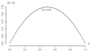
Table 10.2: Relationship Between [latex]\hat p[/latex] and [latex]\hat p (1-\hat p)[/latex].
| [latex]\hat{p}[/latex] | [latex]\hat{p} (1 - \hat{p})[/latex] |
| [latex]0[/latex] | [latex]0 \times (1 - 0) = 0[/latex] |
| [latex]0.2[/latex] | [latex]0.2 \times (1 - 0.2) = 0.16[/latex] |
| [latex]0.5[/latex] | [latex]0.5 \times (1 - 0.5) = 0.25[/latex] |
| [latex]0.8[/latex] | [latex]0.8 \times (1-0.8) = 0.16[/latex] |
| [latex]1[/latex] | [latex]1 \times (1 - 1) = 0[/latex] |
Example: Sample Size Calculation for Proportion
- Determine the sample size n such that we are 95% confident that the error is at most 0.05 when [latex]\hat{p}[/latex] is used to estimate [latex]p[/latex]. Use the conservative estimate [latex]\hat{p}=0.5[/latex].
Since we do not have any extra information about [latex]\hat{p}[/latex], we will use [latex]n = 0.25 \left( \frac{z_{\alpha / 2}}{E} \right)^2[/latex]. [latex]1 - \alpha = 0.95 \Longrightarrow \alpha = 0.05 \Longrightarrow z_{\alpha / 2} = z_{0.025} = 1.96[/latex], and [latex]E = 0.05[/latex].
[latex]n = 0.25 \left( \frac{z_{\alpha / 2}}{E} \right)^2 = 0.25 \times \left( \frac{1.96}{0.05} \right)^2 = 384.16[/latex] rounded up to [latex]n = 385.[/latex]
- Suppose [latex]p[/latex] is known to be in between 0.6 and 0.8. Equipped with this new information, obtain a sample size to ensure the margin of error is at most 0.05 with 95% confidence.
We should take this information into account and use [latex]p_g = 0.6[/latex], the value closest to 0.5 within the range [0.6, 0.8]. Therefore, the required sample size is[latex]n = p_g (1 - p_g) \left( \frac{z_{\alpha / 2}}{E} \right)^2 = 0.6 (1 - 0.6) \times \left( \frac{1.96}{0.05} \right)^2 = 368.79[/latex],
rounded up to [latex]n = 369[/latex].
