13.7 Simple Linear Regression Model (SLRM)
So far, we have focused on a sample of 15 used cars. If we would like to draw conclusions about the population (all used cars), we need some inferential methods. First, we introduce some concepts from conditional probability. Consider, for example, all five-year-old used cars; their prices follow a certain distribution. We call this distribution the conditional distribution of price given age is equal to 5, and the corresponding mean and standard deviation are referred to as the conditional mean and conditional standard deviation. For variables [latex]Y[/latex] and [latex]X[/latex], the conditional mean and standard deviation of [latex]Y[/latex] given [latex]X=x[/latex] are denoted with [latex]\mu_{Y|x}[/latex] and [latex]\sigma_{Y|x}[/latex]. Now, our objective is to model [latex]\mu_{Y|x}[/latex] and the predictor variable [latex]x[/latex] using a straight line (see the figure below). That is
[latex]\mu_{Y|x} = \beta_0 + \beta_1 x[/latex],
where [latex]\beta_0[/latex] and [latex]\beta_1[/latex] are the population intercept and population slope, respectively, with interpretation as follows:
- [latex]\beta_0[/latex]: the average of the response variable [latex]y[/latex] when [latex]x = 0.[/latex]
- [latex]\beta_1[/latex]: the change in the mean value of [latex]y[/latex] when the predictor variable [latex]x[/latex] increases by 1 unit.
For each given value of the predictor variable [latex]x[/latex], the conditional distribution of the response variable [latex]Y[/latex] given [latex]x[/latex] is assumed to follow a normal distribution with a mean [latex]\mu_{\scriptsize Y|x} = \beta_0 + \beta_1 x[/latex] and a standard deviation [latex]\sigma_{y|x} = \sigma[/latex] (that is, the conditional standard deviation of [latex]Y[/latex] is assumed constant for all values of [latex]x[/latex]). For example, most five-year-old cars are not equal in price to the conditional mean [latex]\mu_{y|x=5}[/latex]; [latex]\sigma[/latex] measures the typical difference between the conditional mean [latex]\mu_{y|x=5}[/latex] and the actual value of any given five-year-old car. To capture this variation (sampling error), we introduce an error term [latex]\epsilon[/latex] into the model. The regression model becomes
[latex]Y = \beta_0 + \beta_1 x + \epsilon , \epsilon \sim N(0, \sigma)[/latex].
 |
|
Key Facts: Assumptions for Inferential Methods in Simple Linear Regression
In general, we need the following assumptions to apply the inferential methods in simple linear regression:
- Linearity assumption: There is a linear association between the conditional mean and the predictor variable. This assumption can be checked by plotting a scatter plot ([latex]Y[/latex] against [latex]X[/latex]). If this assumption is met, all the points should roughly lie on a straight line.
- Normal population: Given each value of the predictor variable [latex]x[/latex], the conditional distribution of the response variable is normally distributed. That is, [latex]Y | x \sim N(\beta_0 + \beta_1 x, \sigma)[/latex] or equivalently, the error term [latex]\epsilon[/latex] follows a normal distribution with mean 0 and standard deviation [latex]\sigma[/latex] for all values of [latex]x[/latex].
- Equal standard deviation: The conditional standard deviation of the response variable is the same for all values of the predictor variable [latex]X[/latex]. This common standard deviation is denoted as [latex]\sigma[/latex]. This is equivalent to assuming that the error term [latex]\epsilon[/latex] has the same standard deviation for all values of [latex]x[/latex]
- Independent observations: The observations of the response variable are independent of one another. This is hard to check unless we know how the data were collected.
Checking whether the model assumptions are satisfied or not can be performed by residual analysis. Recall that the residual of the ith observation, [latex]e_i[/latex], is defined as the difference between the observed value ([latex]y_i[/latex]) and the fitted value ([latex]\hat{y}[/latex]), i.e., [latex]e_i = y_i - \hat{y}_i = y_i - (b_0 + b_1 x_i)[/latex]. If the model assumptions are satisfied, the residuals [latex]e_i, i = 1, 2, \dots, n[/latex] can be regarded as a simple random sample from a normal distribution with mean 0 and standard deviation [latex]\sigma[/latex]; this means the residuals should follow an approximate normal distribution with standard deviations that are similar for each value of [latex]x[/latex]. To check the assumptions, we draw two graphs of the residuals:
- Normal population assumption: Draw a Q-Q (normal probability) plot on the residuals. If the normality assumption is met, the points should roughly fall on a straight line.
- Equal standard deviation assumption and linearity assumption: Plot the residuals [latex]e_i[/latex] (y-axis) versus fitted values [latex]\hat{y}_i = b_0 + b_1 x_i[/latex] (x-axis). We can also plot the residuals [latex]e_i[/latex] ([latex]y[/latex]-axis) versus the [latex]x_i[/latex] values ([latex]x[/latex]-axis). If the equal standard deviation assumption is met, we will see a horizontal band centred and symmetric about the line [latex]y[/latex] = 0. If the points form some curvature, the linearity assumption is violated.
Example: Residual Analysis
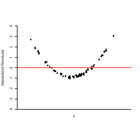
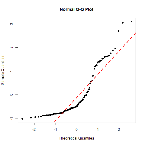
Comment on the following residual plots (first row) and normal probability plots (second row) of three sets of residuals.
 |
 |
 |
 |
 |
 |
| (a) | (b) | (c) |
Figure 13.10: Residual Plots and Normal Probability Plots of Three Sets of Residuals. [Image Description (See Appendix D Figure 13.10)] Click on the image to enlarge it.
- Based on the residuals plot, both the equal standard deviation and the linearity assumptions appear met since the points form a horizontal band centred at 0. According to the normal probability (Q-Q) plot, points are roughly on a straight line and hence the normality assumption is satisfied.
- Based on the residual plot, the linearity assumption appears violated since the residual plot shows “U” shaped curvature. The normal probability plot provides evidence against the normality assumption.
- Based on the residuals plot, the equal standard deviation assumption appears violated since the residual plot does not show a horizontal band. The variation of the residuals gets larger when [latex]x[/latex] increases. The normal probability plot shows that the normality assumption is violated.

Exercise: Residual Analysis for the Used Cars
The residuals for the 15 used cars are given in the following table.
- Given that the least–squares regression line is [latex]\widehat{\text{price}} = 14.118 - 0.9432 \times \text{age}[/latex]. Verify the residual for the first car.
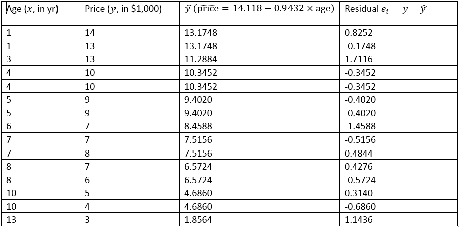
Table 13.2: Fitted Value and Residuals of 15 Used Cars. [Image Description (See Appendix D Table 13.2)] - Comment on the following graphs based on the residuals of the 15 used cars. Explain whether the assumptions for regression inference are met or not.
 |
 |
|
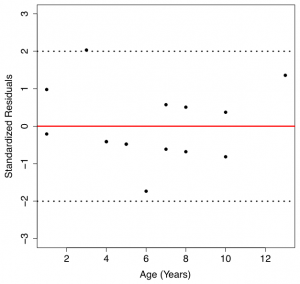
Figure 13.11: Normal Probability Plot of Residuals (Left) and Scatter Plot of Residuals V.S. Predictor Variable (Right) [Image Description (See Appendix D Figure 13.11)] |
|
Show/Hide Answer
Answers:
- Given that the least–squares regression line is [latex]\widehat{\text{price}} = 14.118 - 0.9432 \times \text{age}[/latex], the fitted value for the first used car with age = 1 is [latex]\hat{y}_1 = 14.118 - 0.9432 \times 1 = 13.1748[/latex], and the residual is [latex]e_1 = y_1 - \hat{y}_1 = 14 - 13.1748 = 0.8252[/latex] ($1000), which is the same as the residual given in the table.
- The plot in the left panel is the normal probability plot (normal QQ plot) for the residuals. The points in the QQ plot of the residuals are roughly on a straight line. Therefore, the normal population assumption appears to be met. The plot in the right panel is the scatterplot of residuals (y-axis) versus the predictor variable (x-axis). The points are roughly within a horizontal band centred at 0, without any obvious curvature. Therefore, both the linearity and the equal standard deviation assumptions appear to be met.
