10.2 Distribution of the Sample Proportion

Inferences about the population mean $\mu$ are based on the distribution of the sample mean $\overline{X}$. Similarly, inferences about the population proportion $p$ are based on the distribution of the sample proportion $\hat{p}$.

The population proportion is defined as

$p=\frac{\text{\# of individuals having a certain attribute}}{\text{\# of individuals in the population}}=\frac{\text{\# of successes}}{N}.$

The population proportion can be regarded as a special type of population mean if we let the variable of interest be an indicator variable as follows:

$x_i=\{\begin{array}{ll}1& \text{if the ith individual has the attribute (a success)},\\ 0& \text{if the ith individual does not have the attribute (a failure)}.\end{array}$

Then, the population proportion can be rewritten as

$p=\frac{\text{\# of individuals having a certain attribute}}{\text{\# of individuals in the population}}=\frac{\text{\# of successes}}{N}=\frac{\sum x_i}{N}.$

The variable of interest $X$ has only two possible values: 1 if the individual has the attribute and 0 if not. Randomly select one individual and define $p$ as the probability that this individual has the attribute. As a result, the probability distribution of $X$ is

Table 10.1: Probability Distribution of an Indicator Variable

with a population mean and population standard deviation:

$\mu =\sum xP(X=x)=1\times p+0\times (1-p)=p,$

$\sigma =\sqrt{\sum x^{2}P(X=x)-{\mu }^2}=\sqrt{1^2\times p+0^2\times (1-p)-{\mu }^2}=\sqrt{p-p^2}=\sqrt{p(1-p)}.$

The sample proportion can be viewed as a special type of sample mean (in the same way that the population proportion can be viewed as a special type of population mean). That is, in a simple random sample of size n, the proportion of individuals with the specific attribute is the sample proportion:

$\begin{array}{rl}\hat{p}& =\frac{\text{\# of individuals having a certain attribute in the sample}}{\text{sample size}}\\ & =\frac{\text{\# of successes in the sample}}{n}=\frac{\sum x_i}{n}=\overline{x}\end{array}$

with $x_i=1$ if the individual has the attribute and $x_i=0$ if not.

Recall from Chapter 6, the sampling distribution of the sample mean $\overline{X}$:

• Centre: the mean of the sample mean $\overline{X}$ equals the population mean $\mu$. That is,

  ${\mu }_{\overline{X}}=\mu .$

• Spread: the standard deviation of the sample mean equals the population standard deviation divided by the square root of the sample size. That is,

  ${\sigma }_{\overline{X}}=\frac{\sigma }{\sqrt{n}}.$

These two arguments are true for any population distribution and sample size n.

• Shape:
  • When the population distribution is normal, $\overline{X}$ is also normal regardless of n.
  • When the population distribution is non-normal but the sample size n is large, $\overline{X}$ is approximately normally distributed. This is guaranteed by the central limit theorem (CLT).

The same conclusions can be applied to the sampling distribution of the sample proportion $\hat{p}$, where the variable of interest is

$X=\{\begin{array}{ll}1& \text{with probability }p\\ 0& \text{with probability }1-p\end{array}$

with the population mean $\mu =p$ and standard deviation $\sigma =\sqrt{p(1-p)}$. Therefore, the sampling distribution of the sample proportion $\hat{p}$ is summarized as follows.

Central limit theorem for the sample proportion:

If the sample size n is large enough ($np\ge 5$ and $n(1-p)\ge 5$), the sampling distribution of the sample proportion $\hat{p}$ is approximately normally distributed.

For example, suppose the population proportion is $p=0.05$. Then the sampling distribution of the sample proportion $\hat{p}$ is approximately normally distributed if the sample size is at least

$n=max\{\frac{5}{p},\frac{5}{1-p}\}=max\{\frac{5}{0.05},\frac{5}{1-0.05}\}=max\{100,5.26\}=100.$

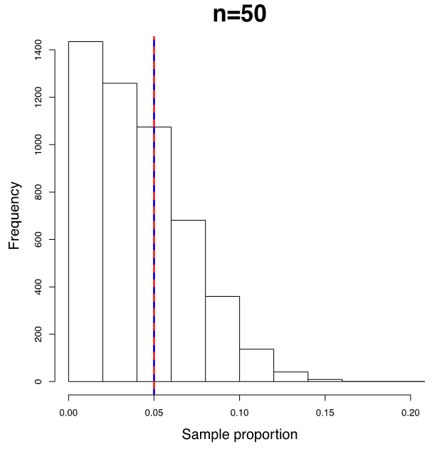
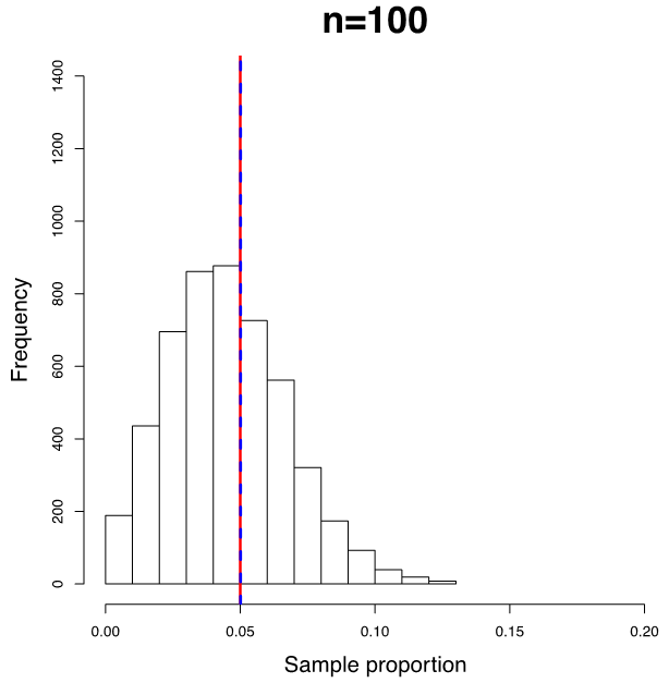
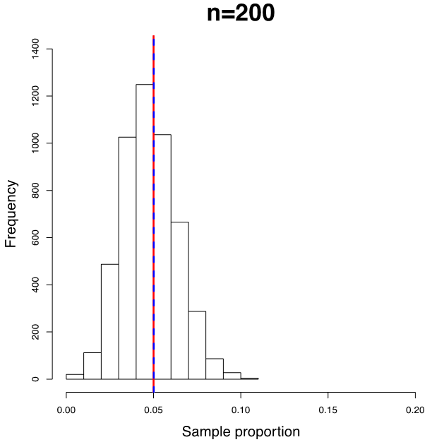
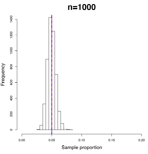
The following figures show the sampling distribution of the sample proportion with $p=0.05$ and sample sizes n = 50, 100, 200, and 1000.

Figure 10.1: Histograms of Sample Proportions with Different Sample Size. [Image Description (See Appendix D Figure 10.1)] Click on the image to enlarge it.

There are several findings:

• The sampling distribution of the sample proportion becomes increasingly normal as the sample size n increases. When n = 50, the sampling distribution of sample proportion is skewed. When n = 100, the distribution is still slightly right skewed. For n = 200 and n = 1000, the sampling distribution appears bell-shaped and symmetric (indicative of a normal distribution).
• The mean of the sample proportion (blue dashed line) is always identical to the population proportion p = 0.05 (red solid line) regardless of the sample size n.
• The standard deviation of the sample proportion decreases as n increases.

To summarize, for $np\ge 5$ and $n(1-p)\ge 5$, $\hat{p}\sim N(p,\sqrt{\frac{p(1-p)}{n}})$. The standardized version of $\hat{p}$ is $Z=\frac{\hat{p}-p}{\sqrt{\frac{p(1-p)}{n}}}\sim N(0,1)$. As a result, inferences about the population proportions are based on the standard normal distribution.